Valuation of Abstract Assets

Valuation of Abstract Assets#

Outline

This lecture introduces some basic financial concepts: abstract assets, the time value of money and interest, and the net present value.

The abstract asset model is a mental model for thinking about the value of assets. An abstract asset is a sequence of current and future discounted cash flows demarcated in some currency, for example, Euros, Dollars, Yuan, or cryptocurrencies such as Bitcoin. On the other hand, cash flows are the inflows and outflows of money from a business or investment and are a key factor in determining the value of abstract assets.
The time value of money is a fundamental concept in finance. It recognizes that money today is worth more than the same amount in the future due to the potential to earn returns or interest over time. Toward this, we also introduced simple and compound interest models which are two methods of calculating interest on loans. Simple interest is calculated on the principal only. Compound interest is calculated on the principal amount and also on the accumulated interest of previous periods and can thus be regarded as interest on interest.
The net present value and the internal rate of return are financial concepts used to determine the current value of future cash flows. They consider the time value of money, recognizing that a dollar today is worth more than a dollar in the future due to the potential for investment.

Introduction#

An abstract asset is the sequence of current and future cash flows demarcated in some currency, for example, Euros, Dollars, Yuan, or cryptocurrencies such as Bitcoin (Fig. 1).

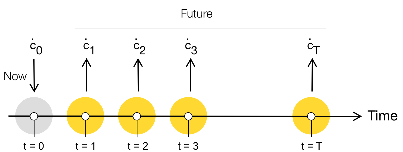
../_images/Fig-Asset-CashFlowDiagram.png — Fig. 1 Abstract asset diagram. During each time period $t=0,2,\dots,T$ an asset has cash flow(s) $\dot{c}_{t}$. The value of the asset is some function $\mathcal{V}$ of these cash flows; the function $\mathcal{V}$ is the called the valuation operator.#

Unfortunately, computing the value of an abstract asset, for example by summing the cashflows $\dot{c}_{t}$ is complicated by the fact that the value of money changes over time (Remark 1):

Remark 1 (Time value of Money)

The value of money is not conserved over time. One dollar today is not worth the same as one dollar tomorrow. The change in the value of money over time is called the time value of money.

Time Value of Money#

The time value of money is an empirical observation that has been seen over hundreds of years. Money is worth more today than the same amount in the future. But why is this the case?

Money given to us today has a greater Utility than the same amount tomorrow, because we have an extra day to invest that money in a risk-free investment, e.g., a savings account or government bond. A risk-free investment is guaranteed to yield a positive return. For example, if we invested $P_{0}$ dollars today in a savings account or government bond, at the end of one investment period, we are guaranteed to have $P_{1}$ dollars:

\[P_{1} = (1+i)\cdot{P_{0}}\]

where $i>0$ is the risk-free interest rate. Thus, if given a choice between $P_{0}$ dollars today and the same amount one investment period in the future, a rational investor would always choose to take the $P_{0}$ dollars now.

By taking $P_{0}$ dollars today, you could invest those dollars risk-free and get $P_{1} = (1+i)\cdot{P_{0}}$ back, where $P_{1}>P_{0}$. Thus, the only case where it makes sense to take the future money is negative interest $i\leq{0}$ which is forbidden by the condition $i>0$.
This scenario assumes a risk-free investment that always pays an interest rate $i>0$, but a truly risk-free investment is only a theoretical concept. However, risk-free investments, and the risk-free rates of return i are often approximated by US Treasury debt securities.

Interest models#

Interest represents the cost of borrowing money or the return on lending money. Simple and compound interest are two types of interest that significantly impact investment growth and borrowing costs, making them critical factors to consider when making financial decisions.

Simple interest is paid only on the initial principle. For example, if amount $A(0)$ is invested in an interest-bearing savings account at t=0 with a simple interest rate of $r$ per period, then the account will hold $A(n)$ after $n$ periods:

(1)#\[A(n) = A(0)\cdot\left(1+rn\right)\]

The interest earned is not reinvested, and thus the interest earned is constant over time. However, compound interest considers both the principal and the interest accumulated over time, i.e., you earn interest on your interest. For example, if amount $A(0)$ is invested into an interest-bearing savings account that pays a compound interest rate $r$ per period, then after $n$ periods the account would hold $A(n)$:

(2)#\[A(n) = A(0)\cdot\left(1+r\right)^n\]

As the number of periods become large, compound interest always outperforms simple interest (Fig. 2).

../_images/Fig-Simple-Compound-Balance.svg — Fig. 2 Simple versus compound interest for n-periods for an interest rate of $r = 0.05$ per-period. Compound interest outperforms simple interest as the number of periods becomes large.#

Finally, interest rates are typically quoted as annualized values and can be compounded at different rates, e.g., annually, quarterly, monthly, etc, and compound interest can be computed on a discrete or continuous basis (Definition 1):

Definition 1 (Discrete and continuous compounding)

Let there be n-compounding periods per year and an annualized interest rate of r-percent. Then an initial investment $A(0)$ will be worth:

(3)#\[A(m) = A(0)\cdot\left(1+r/n\right)^{mn}\]

after m-years where the interest rate r is a decimal. As the number of compounding periods $n\rightarrow\infty$, the investment $A(m)$ approaches the continuous compounding limit:

(4)#\[\lim_{n\rightarrow\infty}A(m) = A(0)\cdot\exp\left(rm\right)\]

Simple versus Compound Interest

We’ll exclusively deal with compound interest throughout this course, as this is the mechanism used in the real world for different types of investments.

Discrete discounting#

Now that we have established money’s present value is higher than its future value, we need a way to compare money from different time periods. A useful model for the time value of money is to think of money from different time periods as being in different currencies that must be exchanged. To compare money or cash flows from different time periods, we use the equivalent of an exchange rate, which we call the discount factor.

Suppose we wanted to convert the value of a cashflow from one time period in the future into today’s dollars, i.e., we discount the future value of cashflow to its present value. To do this, we use a one-period discrete (finite) conversion (Definition 2):

Definition 2 (One Period Discrete Conversion)

For any one-step finite period $t\rightarrow{t+1}$, the present value of cashflow denoted as $\dot{c}_{t}$ and the future value of cash-flow denoted by $\dot{c}_{t+1}$ are related by the expression:

(5)#\[\dot{c}_{t+1} = \left(1+r_{t+1,t}\right)\cdot{\dot{c}_{t}}\]

where $r_{t+1,t}>{0}$ is the discount rate for period $t\rightarrow{t+1}$.

The term $(1+r_{t+1,t})$, which denotes the hypothetical exchange rate between the present $\dot{c}_{t}$ and future $\dot{c}_{t+1}$ cashflows for the period $t\rightarrow{t+1}$, is called the discrete discount factor.
The discrete discount factor is always greater than one, thus $\dot{c}_{t+1}>\dot{c}_{t}$ for any $t$.

Let’s do an example to illustrate one-period conversions (Example 1):

Example 1 (Present value of a future coffee)

Someone offers to buy you a coffee tomorrow (one time period in the future) for $\dot{c}_{1}$ = 3.35 USD. What is the current value $\dot{c}_{0}$ of the coffee if the discount rate is $r_{1,0}=10\%$?

Solution: Rearranging Eqn. (5) for the current value of the coffee $\dot{c}_{0}$ gives:

\[\dot{c}_{0} = \frac{\dot{c}_{1}}{1+r_{1,0}}\]

Subsutituing $r_{1,0}=10\%$ and $\dot{c}_{1}$ = 3.35 USD says the current value of your future coffee is: $\dot{c}_{0}$ = 3.05 USD.

Suppose we have a project that spans multiple time periods. We can develop a multi-period conversion by sequentially applying one-period calculations. Let’s start with period zero to period one:

\[\dot{c}_{1} = \left(1+r_{1,0}\right)\cdot\dot{c}_{0}\]

Then, period one to period two is given by:

\[\dot{c}_{2} = \left(1+r_{2,1}\right)\cdot\dot{c}_{1}\]

but we can substiture $\dot{c}_{1}$ into the expression above to give:

\[\dot{c}_{2} = \Bigl[\left(1+r_{2,1}\right)\left(1+r_{1,0}\right)\Bigr]\cdot\dot{c}_{0}\]

Doing this computation between 2 and 3, and then 3 to 4, etc, we develop a relationship between the current value of cash flow $\dot{c}_{0}$ and the future value of cash flows $\dot{c}_{t}$ over multiple periods (Definition 3):

Definition 3 (Multiple period discrete discounting)

Let $\dot{c}_0$ be the present cashflow, and $\dot{c}_t$ be the future cashflow in period $t$. Let $r_{j+1,j}$ represent the discount rate between discrete time periods $j$ and $j+1$. Then:

(6)#\[\dot{c}_{t} = \left[\prod_{j=0}^{t-1}\left(1+r_{j+1,j}\right)\right]\cdot\dot{c}_{0}\qquad{t=1,2,\dots,T}\]

The product term is the multi-period discount factor which we defined as the function $\mathcal{D}_{t,0}(r)$.

Equation (6) can be written in a more compact form as:

\[\dot{c}_{t} = \mathcal{D}_{t,0}\cdot\dot{c}_{0}\qquad{t=1,2,\dots,T}\]

In the particular case where discount rates $r_{j+1,j}$ are equal in each period (let’s call this value $\bar{r}$), the multi-period discount factor becomes:

(7)#\[\mathcal{D}_{t,0} = (1+\bar{r})^{t}\qquad{t=1,2,\dots,T}\]

Let’s do an example of multi-period discounting (Example 2):

Example 2 (Multiple period discount)

Compute the present value of $1 collected $T$ time units into the future for a constant discount rate of 2%, 4%, 6%, 8%, and 10% per time period.

Solution: The value of money today is the present value, whereas the value of money T time periods is the future value. The quantity $\dot{c}_{0}$ is the present value, while $\dot{c}_{i},i=1,2,\dots,T$ denotes future value. To compute the present value of $1 collected T time units in the future, we solve Eqn. (6) for $\dot{c}_{0}$ in terms of the future value $\dot{c}_{i},i=1,\dots,T$ and the discount factor $\mathcal{D}$:

\[\dot{c}_{0} = \mathcal{D}_{i,0}^{-1}\cdot\dot{c}_{i}\qquad{i=0,1,\dots,T}\]

where $\mathcal{D}_{i,0}^{-1}$ is given by:

\[\mathcal{D}_{i,0}^{-1} = \frac{1}{(1+\bar{r})^{i}}\qquad{i=0,1,\dots,T}\]

We assumed a constant discount rate $r$ between now (i = 0) and $i = T$ time units into the future. Given that we are looking at the present value of $1, we can set $\dot{c}_{i} = 1$ USD:

\[\dot{c}_{0} = \frac{\dot{c}_{i}}{(1+\bar{r})^{i}}\qquad{i=0,1,\dots,T}\]

../_images/Fig-PresentValue-FuturePayment.pdf — Fig. 3 Present value (PV) of $1 USD collected T periods in the future as a function the discount rate $r$.#

Continuous discounting#

Previously we used a discrete finite time difference, e.g., days, weeks, or even years, to compute the discount factor. However, suppose the time difference for each period was infinitesimally small, i.e., the time difference was continuous. In this case, we have continuous discounting, where the discount factor $\mathcal{D}(r,t) = \exp\left(r\cdot{t}\right)$ gives a future value expression of the form:

(8)#\[\dot{c}_{t}= \exp\left(r\cdot{t}\right)\cdot\dot{c}_{0}\]

where $r>0$ denotes the instantaneous discount rate, and t denotes the time. Let’s do a continuous discount factor example (Example 3):

Example 3 (What is $1 collected today worth T years from now? )

Suppose we are given $1 dollar today. What is the future value of $1 T periods from now for an instantaneous discount rate of $r$ = 2%, 4%, 6%, 8% and 10% and continuous discounting? Plugging these values in (8) gives:

../_images/Fig-FutureValue-1-dollar.pdf — Fig. 4 Future value (FV) of 1 USD (today) T-periods in the future using a continuous discounting model.#

Julia script to compute the future value as a function of the discount rate $r$, and plot the data:

# load packages (assume these are installed)
using Plots
using Colors

# setup color dictionary -
# Colors taken from: https://personal.sron.nl/~pault/
colors = Dict{Int64,RGB}()
colors[1] = colorant"#0077BB" 
colors[2] = colorant"#33BBEE"
colors[3] = colorant"#009988"
colors[4] = colorant"#EE7733"
colors[5] = colorant"#CC3311"
colors[6] = colorant"#EE3377" 
colors[7] = colorant"#BBBBBB"

# initialize -
Cₜ = 1.0;
R = [0.02, 0.04, 0.06, 0.08, 0.10];
number_of_periods = 25;
number_of_rates = length(R)
Cₒ = Array{Float64,2}(undef, number_of_periods, number_of_rates + 1);

# main loop - compute the present values
for j ∈ 1:number_of_rates
        
    # pick a rate -
    r = R[j];

    # iterare of period -
    for i ∈ 1:number_of_periods
        
        # compute the discount -
        D = exp(r*i)

        # compute the future values
        Cₒ[i,1] = i-1       # period is in the first col
        Cₒ[i,j+1] = (D)*Cₜ   # future value is for each r in the col 2,... 
    end
end

# plot -
for i ∈ 1:number_of_rates
    plot!(Cₒ[:,1],Cₒ[:,i+1], c = colors[i], label="r = $(R[i])", lw=2, xlim=(0.0,number_of_periods), ylim=(0.0,14.0),
        bg="floralwhite", background_color_outside="white", framestyle = :box, 
        fg_legend = :transparent)
end
current();
xlabel!("Period index (AU)", fontsize=18)
ylabel!("Future value (USD)", fontsize=18)

Net present value#

Now that we can calculate the time value of money, let’s revisit valuing abstract assets. The simplest method to value an abstract asset is to compute the net cash flow for each time period and discount that cashflow to the present value. Suppose, at node t=k, we have $\mathcal{S}_{k}$ cash streams entering or leaving the asset time node. The net cash flow at node t=k, denoted by $\bar{c}_{k}$, is given by:

\[\bar{c}_{k} = \sum_{s\in\mathcal{S}_{k}}\nu_{s}\dot{c}_{s}\]

where $\nu_{s}$ is a direction parameter; $\nu_{s}=+1$ if stream s enters node t=k, while $\nu_{s}=-1$ if stream s exists node t=k. We then sum all the current and future cash flows and convert them to a shared basis for comparison, e.g., current dollars. This discounted sum is called the Net Present Value (NPV) (Definition 4):

Definition 4 (Net Present Value)

The net present value NPV is the sum of current and future cash flows, discounted to current dollars:

\[ \begin{equation} \text{NPV}(T,r) = \sum_{i=0}^{T}{\mathcal{D}_{i,0}^{-1}}(r)\cdot\bar{c}_{t} \end{equation} \]

where the quantity $\bar{c}_{t}$ denotes the net cash flow in time period t, the quantity T is the number of time periods (lifetime of the project or investment), and $\mathcal{D}_{i,0}(r)$ is the multistep discount factor, with discount rate(s) r.

The discount factor $\mathcal{D}_{i,0}(r)$ can be modeled as either a discrete or a continuous discount factor.
The discount $\mathcal{D}_{0,0}(r) = 1$ for all values of $r$.

Decisions#

The net present value is often used as a decision tool to rank a particular project or investment against alternative investments. In this context, the discount rate $r_{t+1,t}$ represents the minimum rate of return that a decision-maker would accept for a project or investment. To evaluate a project or investment, we use the following decision criteria:

NPV < 0: A negative NPV indicates the proposed asset or project will generate a loss over the time horizon of the project at the given discount rate. The decision-maker should consider alternative investments.
NPV = 0: A zero NPV indicates the proposed project will breakeven over the time horizon of the project at the given discount rate. The decision-maker is indifferent to the project.
NPV > 0: A positive NPV indicates the proposed project will generate a positive return over the time horizon of the project at the given discount rate. The decision-maker should consider choosing the proposed project.

The NPV decision rule relies on computing the sum of discounted future cash flows. However, in these calculations, what discount rate should we use? This question is difficult; the correct discount rate varies between applications and industries and is subjective to the decision-maker.

Let’s consider an example to illustrate the NPV decision rule concerning the installation of an upgraded lighting system in a building (Example 4):

Example 4 (Should we upgrade our lighting system?)

Johnson Controls offers to install a new computer-controlled lighting system that will reduce electric bills by 90,000 USD in each of the next three years. The system costs 230,000 USD and takes 1-year to install. The building owner has a r̄ = 4% discount rate per year (constant for the lifetime of the project). Should the owner install the system?

Solution: Let’s assume a discrete discount factor model and compute the net present value of the project.

If the net present value is positive, the owner should install the system:
If the net present value is negative, the owner should not install the system.

The Julia code to compute the net present value of the project is shown below:

cashflows = [-230,90,90,90];
number_of_periods = length(cashflows);
discounted_cashflows = Array{Float64,1}(undef, number_of_periods);
r̄ = 0.04; # 4% discount rate

# compute the discounted cash flows -
for i ∈ 0:(number_of_periods - 1)
    discounted_cashflows[i+1] = cashflows[i+1]/((1+r̄)^i);
end
NPV = sum(discounted_cashflows);

The net present value of the project is NPV = 19.75k at a discount rate of r̄ = 0.04. Since the net present value is positive, we should consider installing the upgraded lighting system in the building.

source: The Johnson Controls example was modified from MIT 15.401.

Internal Rate of Return#

At a minimum, a decision-maker should be indifferent to a project or investment, i.e., the project or investment should at have (at least) a value of NPV = 0. The discount rate $r^{\star}$ where the net present value for a project or investment is equal to zero is called the Internal Rate of Return (IRR) (Definition 5):

Definition 5 (Internal Rate of Return)

The internal rate of rerturn IRR is the effective (constant) discount rate $r^{\star}$ that makes the net present value of a project or investment equal to zero:

\[ \begin{equation} \sum_{t=0}^{T}{\mathcal{D}_{t,0}^{-1}}(r^{\star})\cdot\bar{c}_{t} = 0 \end{equation} \]

where $\mathcal{D}_{t,0}(r^{\star})$ is the discount factor between the current period and a future period $t$ using the discount rate $r^{\star}$, and T denotes the number of periods (lifetime of the project or investment).

The discount factor $\mathcal{D}_{i,0}(r)$ can be modeled using either a discrete or a continuous compounding model.
The IRR assumes that discount rate is constant over the lifetime of the project or investment.

Like the NPV, the IRR can be thought of as a decision boundary of sorts; the IRR is the discount rate where the project manager or investor is indifferent to the project or investment. Thus, we can formulate the following decision criteria:

If the project discount rate is greater than the IRR, the project or investment is not attractive, i.e., NPV < 0. The decision-maker should consider alternative investments or projects.
If the project discount rate is less than the IRR, the project or investment is attractive, i.e., NPV > 0. The decision-maker should consider the project or investment.

Let’s revisit the lighting example, and compute the internal rate of return for the proposed project (Example 5):

Example 5 (Internal rate of return for the lighting project)

Johnson Controls offers to install a new computer-controlled lighting system that will reduce electric bills by 90,000 USD in each of the next three years. The system costs 230,000 USD and takes 1-year to install. Compute the internal rate of return $r^{\star}$ for this project and determine if we should install the upgraded system.

Solution: For this problem we estimate the internal rate of return $r^{\star}$ by minimzing the squared net present value. The Julia code to compute the IRR, which uses the Optim.jl package, is given by:

# load external packages -
using Optim

# define the loss function (we are minimizing the squared NPV)
function loss(r̄::Float64, cashflows::Array{Float64,1})
    
    # initialize -
    number_of_periods = length(cashflows);
    discounted_cashflows = Array{Float64,1}(undef, number_of_periods);
    
    # main -
    for i ∈ 0:(number_of_periods - 1)
        discounted_cashflows[i+1] = cashflows[i+1]/((1+r̄)^i);
    end

    # compute the NPV -
    NPV = sum(discounted_cashflows);

    # return -
    return (NPV)^2
end

# solve using the optimize method from Optim.jl -
cashflows = [-230.0,90.0,90.0,90.0];
objective(x) = loss(x, cashflows);
soln = optimize(objective, 0.0, 0.20)
r̄ = soln.minimizer;

The internal rate of return for the lighting project equals IRR = 0.082. Since the internal rate of return is greater than the discount rate r̄ = 0.04, the building owner should install the upgraded lighting system.

Alternative investments?#

When considering net present value, people often wonder about hypothetical alternative investments. If a project has a negative net present value, it is not attractive. However, if a project has a zero or positive net present value, the decision can be subtle because another project or investment could exist that offers a better return. Answering this question is impossible, but we can imagine a minimum hypothetical investment, which is a risk-free investment with the same time-to-maturity as the project.

For any project with a positive net present value, the income generated should be equal to or greater than that of a risk-free investment with the same time-to-maturity, such as a zero-coupon bond or a certificate of deposit (CD). Later on, we will discuss U.S. Treasury bills, notes, and bonds. For now, consider a zero-coupon treasury bond as a guaranteed risk-free investment with a fixed interest rate. Therefore, instead of investing in a project with upfront costs and future cash flows, we could invest the upfront costs in a zero-coupon bond with the same time-to-maturity as the project. If the net present value of a project is less than that of a zero-coupon bond, the project is not attractive as we would be risking capital without earning a premium for the additional risk.

Summary#

In this lecture, we introduced:

The abstract asset model is a mental model for thinking about the value of assets. An abstract asset is a sequence of current and future discounted cash flows demarcated in some currency, for example, Euros, Dollars, Yuan, or cryptocurrencies such as Bitcoin. On the other hand, cash flows are the inflows and outflows of money from a business or investment and are a key factor in determining the value of abstract assets.
The time value of money is a fundamental concept in finance. It recognizes that money today is worth more than the same amount in the future due to the potential to earn returns or interest over time. Toward this, we also introduced simple and compound interest models which are two methods of calculating interest on loans. Simple interest is calculated on the principal only. Compound interest is calculated on the principal amount and also on the accumulated interest of previous periods and can thus be regarded as interest on interest.
The net present value and the internal rate of return are financial concepts used to determine the current value of future cash flows. They consider the time value of money, recognizing that a dollar today is worth more than a dollar in the future due to the potential for investment.