Functions, Control Statements, Recursion and Testing

Overview

This lecture will explore some essential programming tools that will allow us to write more complex programs. We will introduce functions, control statements, recursion, error-handling patterns, and unit testing.

• Functions are blocks of code that perform specific tasks and may return a value.

• Control statements are programming constructs that allow you to control the flow of execution of your code; further, they will enable you to create loops that repeat a block of code until a particular condition is met.

• Recursion is a programming technique where a function calls itself with a simplified version of the original problem until the problem is small enough to be solved directly. Recursion is an essential concept in programming. It solves many problems, including search and sorting problems and problems involving recursive data structures such as trees and linked lists.

• Error handling allows functions to respond to the unexpected. When an unexpected condition occurs, a function may be unable to return a reasonable value to its caller. However, error-handling patterns allow functions to respond gracefully.

• Unit tests are a way to test your code to ensure it works as expected. Unit tests are a critical part of the development process because they allow you to test your code as you write it, which can help you catch bugs early on and avoid wasting time debugging later. They also can be used to test your code after you have made changes to it, which can help you catch bugs that your changes may have introduced.

---

Functions

In programming, a function is a block of code that performs a specific task and may return a value. Functions are a fundamental building block of most programming languages, and they are used to modularize and organize code into reusable units. Functions allow you to write code that can be called from multiple places in your program, making your code more organized, modular, and easier to read and maintain. Functions can also accept input in the form of arguments, which are values passed to the function when it is called, and they can return a value to the caller using the return statement. Functions can be defined and called from anywhere in your program and can be called multiple times with different arguments. Thus, they are essential for organizing and modularizing code in any programming project.

Mathematical functions

Most of us are familiar with the idea of a function from mathematics (Fig. 3). A mathematical function takes input from a domain (the set of possible inputs) and converts this input to an output that lives in the codomain. The codomain is the set of all possible output values, while the range (a subset of the codomain) is the set of values we observe.

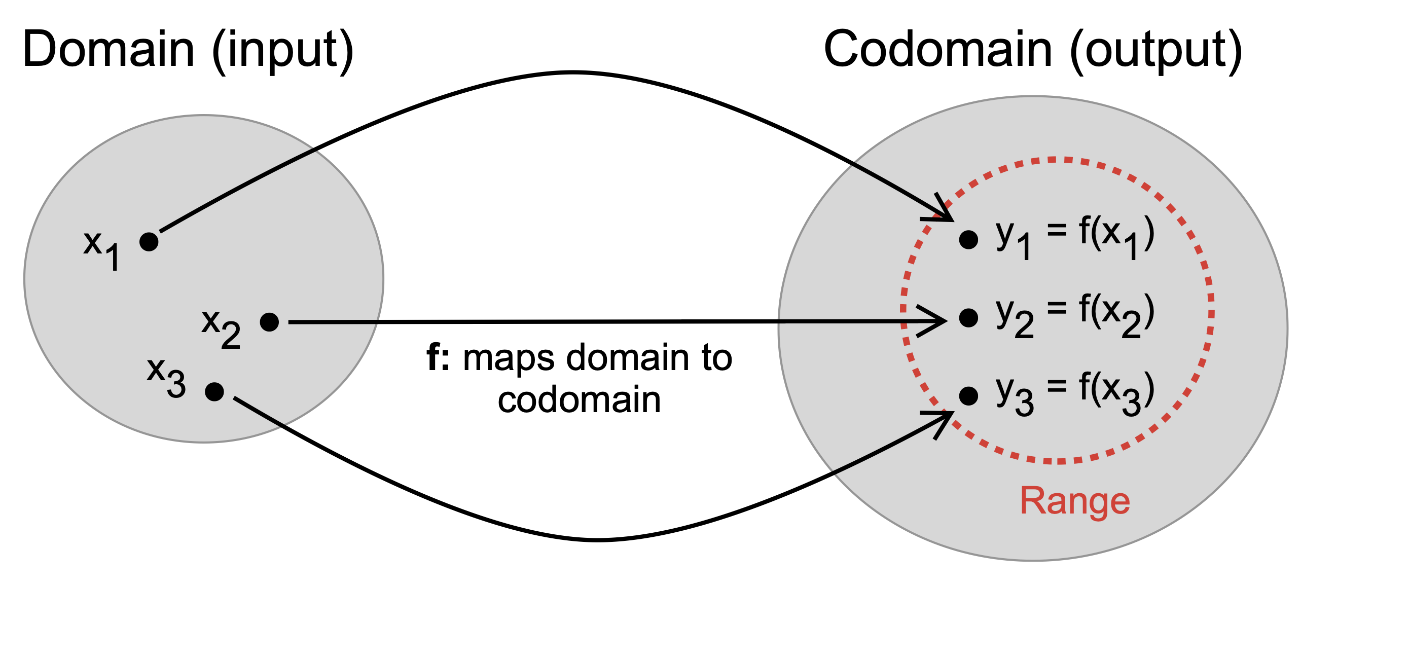
Fig. 3 Schematic of a function from mathematics. A function takes a tuple of inputs and maps them to a tuple of outputs. The function \(f\) maps the input \(x\) to the output \(y\).

Formally a mathematical function is defined as (Definition 2):

Definition 2 (Mathematical function)

In mathematics, a function from a set \(X\) to a set \(Y\) assigns to each element of \(X\) exactly one element of \(Y\). The set \(X\) is the domain of the function, while the set \(Y\) is called the codomain of the function. A function, its domain, and its codomain, are declared using the notation:

\[f:X\rightarrow{Y}\]

where the value of a function \(f\) at an element \(x\in{X}\), denoted by \(f(x)\), is called the image of \(x\) under \(f\), or the value of \(f\) applied to the argument \(x\).

The function \(f\) is the rule that describes how the inputs are transformed into results, while \(y = f(x)\) denotes the output value in the range of the function \(f\).

Functions on the computer

Functions on the computer share many of the features of mathematical functions, but there are a few crucial differences. For example, on the computer, a function is an object that maps a tuple of arguments to a tuple of return values. However, unlike mathematical functions, computer functions in languages such as Julia, Python, or the C-programming language can alter (and be affected by) the global state of your program.

The basic syntax for defining functions in Julia, Python or the C-programming language involves defining a function name, the set of input (positional or keyword) arguments, the return value types, and finally, the logic (called the function body) required to transform the input arguments to the return values:

julia

"""
    linear(x::Number, m::Number, b::Number) -> Number

Compute the linear transform of the scalar number `x` given values for the slope `m` and intercept `b` parameters. 
All arguments are of type `Number`
"""
function linear(x::Number, m::Number, b::Number)::Number
    
    # check: are x, m and b Real numbers?
    # ...

    # compute the linear transform of the x-value
    y = m*x+b

    # return y 
    return y
end

python

def linear(x,m,b):

    # linear transform the x-value
    y = m*x+b

    # return y 
    return y

C

double linear(double x, double m, double b) {

    /* define and initialize y */
    double y = 0.0;
    
    /* Linear transform the x-value to y */
    y = m*x + b;

    /* return y */
    return y;
}

Let’s compare and contrast the structure of a simple function named linear, which computes a linear transformation written in Julia, Python and the C-programming language.

The different implementations of the linear function share common features:

• Each implementation has a return y statement at the end of the function body. A return statement tells the program (which is calling your function) that the work being done in the function is finished, and here is the finished value.

• The implementation of the math \(y = mx+b\) looks strikingly the same in each language; there is a conserved set of operations, e.g., the addition + and multiplication * operators defined in each language which are similar across many languages.

However, many features are different in the linear function implementation between the languages:

• Julia functions start with the function keyword and stop with an enclosing end keyword. Functions in the C-programming language begin with the return type, and the function body is enclosed in braces {...}. Functions in Python start with the def keyword followed by the name, arguments, and a colon, while the return statement marks the end of a Python function; there is no other closing keyword or character.

• Functions in the C-programming language strictly require type information about the arguments, but neither Julia or Python requires this information; it is recommended in Julia but not required, and while newer Python versions have support for typing, the Python runtime does not enforce function and variable type annotations.

• The C-programming language requires that variables be defined before they are used, while both Julia and Python do not require this step.

Arguments: Pass by sharing

Julia function arguments follow the’ pass-by-sharing’ convention, i.e., values passed into functions as arguments are not copied. Instead, function arguments act as new variable bindings (new locations that can refer to values), but the underlying values they refer to are identical to the passed values (Remark 2):

Remark 2 (Pass-by-sharing)

The pass-by-sharing paradigm leads to interesting (and sometimes confusing) side effects: Modifications made to mutable values within the function body are visible to the caller (outside the function).

This behavior is found in many other languages such as Scheme, Lisp, Python, Ruby, and Perl.

Arguments: Default and keyword arguments

Providing sensible default values for function arguments is often possible (and desirable). Providing default values saves users from passing every argument on every call. Let’s re-write the linear function with default values for the function arguments:

"""
    linear(x::Number, m::Number = 0.0, b::Number = 0.0) -> Number

Compute the linear transform of the scalar number `x`
"""
function linear(x::Number, m::Number = 0.0, b::Number = 0.0)::Number
    
    # linear transform the x-value
    y = m*x+b

    # return y 
    return y
end

# call: we can call with only *two* args
y = linear(2.0,3.0) # this should return 6

Some functions need a large number of arguments or have a large number of behaviors. Remembering how to call such functions can take time and effort. Keyword arguments make these complex interfaces more accessible and extend by allowing arguments to be identified by name instead of by position. For example, consider the linear function written with keyword arguments:

"""
    linear(x::Number; slope::Number = 0.0, intercept::Number = 0.0) -> Number

Compute the linear transform of the scalar number `x` given values for 
the `slope` and `intercept` keyword arguments. All arguments are of type `Number`
"""
function linear(x::Number; slope::Number = 0.0, intercept::Number = 0.0)::Number
    
    # map keyword values to previous parameters
    m = slope
    b = intercept

    # linear transform the x-value (set to y)
    y = m*x+b

    # return y 
    return y
end

# call: we can call with 1, 2 or 3 args
y = linear(2.0; slope = 2.0, intercept=0.1) # this should return 4.1

Functions as contracts

A function can also be considered a contract between a developer and a user. The developer defines the function and specifies how it should behave, while the user relies on it to perform as described. The developer ensures that the function is written correctly and behaves as intended, while the user is responsible for providing the correct input and understanding the output. To facilitate this contract, consider a few items:

• A well-defined function must have clear input and output specification documentation, making it easy for the user to understand. Clear and informative documentation is critical to promoting efficient and effective communication between the developer and the user and can help the user trust the developer’s work.

• Function naming is also critical because it helps to communicate the function’s purpose and behavior clearly and accurately.

• Finally, good variable and constant names make your code more readable and understandable. They make it easier for other developers (and even you) to understand what the variable or constant represents just by reading its name.

Control statements

Control statements are an essential part of programming. Control statements allow you to create programs that make decisions and perform tasks based on certain conditions. Control statements are programming constructs that will enable you to control the flow of execution of your function. They allow you to specify conditions under which a particular block of code should be executed and will allow you to create loops that repeat a block of code until a specific condition is met. Let’s explore some common control statements that you will routinely use in your functions and programs:

• If-else conditional statements allows you to execute different logic branches based on a Bool condition.

• Iteration allows you to execute a code block many times.

If-else conditional statements

A common programming task is to check whether a condition is true or false and then execute code depending on this condition; this is a called conditional evaluation. Conditional evaluation, which is a important structure in almost all programming languages, is encoded with if-else statements.

Conditional evaluation allows portions of code to be evaluated or not evaluated depending on the value of a boolean expression. Let’s consider the anatomy of the if-elseif-else conditional syntax in Julia, Python and the C-programming language:

julia

if condition_1
    # code statememts executed if condition_1 == true
elseif condition_2
    # code statememts executed if condition_2 == true
else
    # code statememts executed if condition_1 == false AND condition_2 == false
end

python

if condition_1:
    # code statements executed if condition_1 == true
elif condition_2:
    # code statememts executed if condition_2 == true
else: 
    # code statements executed if condition_1 == false AND condition_2 == false

C

if (condition_1) {
  /* block of code to be executed if condition_1 is true */
} else if (condition_2) {
  /* block of code to be executed if condition_2 is true */
} else {
  /* code statements executed if condition_1 == false AND condition_2 == false */
}

The conditions in the if-else pseudo code above are statements that evaluate to Bool values. These statements can be single expressions like \(x\geq{y}\), and function calls that return a Bool type, or compound expressions containing several cases, e.g., \(x\geq{y}\) and \(x\leq{z}\).

To facilitate the compound chaining of logical statements, most programming languages, including Julia, define short-cut logical operators:

• The && operator corresponds to the logical AND operator. The && operator in Julia performs a logical AND operation between two operands. In a logical AND operation, if both operands are true, the result is true. If either operand is false, the result is false.

• The || operator corresponds to the logical OR operator. The || operator in Julia performs a logical OR operation between two operands. In a logical OR operation, if either operand is true, the result is true. If both operands are false, the result is false.

Let’s see a few examples of && and || operators:

# Test: && operator

# set some constants
x = 5.0;
y = 10.0;

# if statement
if (x > 0 && y > 0)
    println("Both x and y are greater than zero")
else
    println("Either x or y is less than zero")
end

Both x and y are greater than zero

The if-else statements which use the logical OR short-cut operator || are similar:

# Test: && operator

# set some constants
x = -5.0;
y = 1.0;

# if statement
if (x > 0 || y > 0)
    println("Either x OR y is greater than zero")
else
    println("Both x and y are less than zero")
end

Either x OR y is greater than zero

Iteration

A typical programming operation is repetitively performing a task using a list of items. For example, finding the sum of a list of experimental values to estimate a mean value, translating words in an article from one language to another, etc. This type of operation is called iteration. Two common approaches to performing iteration are resident in almost all programming languages, For-loops and While-loops.

For-loops

For-loops, which date back to the late 1950s and are key language constructs in all programming languages, execute a block of code a fixed number of times. For-loops have two parts: a header and a body:

• The header of a for-loop defines the iteration count, i.e., the number of times the loop will be executed. In modern for-loop header implementations, Iterators provide direct access to the items in a list instead of the item’s index.

• The body holds the code that is executed once per iteration. A for-loop header typically declares an explicit loop counter or loop variable, which tells the body which iteration is being performed. Thus, for-loops are used when the number of iterations is known before entering the loop.

Let’s look at the structure and syntax of a for-loop in Julia, Python, and the C-programming language where we are iterating over a fixed range of values:

julia

for i in 1:10 # gives i values from 1 to 10 inclusive
    
    # loop body: holds statements to be executed at each iteration
    println("i = $(i)")
end

python

for i in range(1, 10):  # gives i values from 1 to 9 inclusive (but not 10)
    
    # loop body: holds statements to be executed at each iteration
    print("i = "+str(i)) # why str()?

C

/* Using for-loop iteration range 0 -> 9 */
for (int i = 0; i < 10; i++) {
    
    /* body: holds statements to be executed at each iteration */
    printf("i = %d\n",i);
}

Let’s illustrate the for-loop and functions by developing a function that iteratively computes Fibonacci numbers (Example 6):

Example 6 (Fibonacci sequence for-loop)

Develop a fibonacci_for_loop function which takes an integer \(n\) as an argument and returns the Fibonacci sequence.

Solution: The Fibonacci numbers, denoted as \(F_{n}\), form a sequence, the Fibonacci sequence, in which each number is the sum of the previous two numbers:

\[F_{n} = F_{n-1}+F_{n-2}\qquad{n\geq{2}}\]

where \(F_{0} = 0\) and \(F_{1} = 1\). A Julia implementation of the fibonacci_for_loop function is given by:

"""
    fibonacci(n::Int64) -> Array{Int64,1}

Computes the `fibonacci` sequence for 0 to n where n >= 1

See: https://en.wikipedia.org/wiki/Fibonacci_number
"""
function fibonacci_for_loop(n::Int64)::Array{Int64,1}


    # check: is n legit? n>=1
    # ...

    # initialize -
    sequence = zeros(n+1); # why n+1 (and not n)?

    # we know the first two elements -
    sequence[1] = 0;
    sequence[2] = 1;

    # main loop -
    for i in 3:(n+1)
        sequence[i] = sequence[i-1] + sequence[i-2]
    end

    # return -
    return sequence
end 

Iterators

In the discussion and examples above, for-loops used a loop counter to iterate through a list of items. However, many modern languages, e.g., Julia, Python, Swift or Rust implement the for-in loop pattern. A for-in loop pattern directly iterates through the elements of a list without a loop counter. Let’s do an example. Imagine we have a list of chemical names stored in a collection named list_of_chemicals. A for-in construct allows us to iterate through the list directly without using a loop counter:

julia

# define list of chemicals -
list_of_chemicals = ["alpha-D-glucose", "alpha-D-glucose-6P", "beta-D-Fructose-6P"]

for chemical in list_of_chemicals # gives each chemical in the list
    # loop body: holds statements to be executed at each iteration
    println("Name of chemical: $(chemical)")
end

python

# define list of chemicals -
list_of_chemicals = ['alpha-D-glucose', 'alpha-D-glucose-6P', 'beta-D-Fructose-6P']

for chemical in list_of_chemicals:  # gives each chemical in the list
    # loop body: holds statements to be executed at each iteration
    print("Name of chemical:"+chemical)

While-loops

A while-loop is a control structure that repeats a block of code in the loop’s body as long as a particular condition, which is encoded in the loop’s header, is true.

The header of a while-loop evaluates a Boolean control expression that determines whether the body is executed or the loop terminates. If the control expression evaluates to true, the code in the body is executed; otherwise, the loop terminates. Thus, unlike a for-loop that iterates over a specified range of values, a while-loop can repeat both for a fixed number of iterations or indefinitely, depending upon the result of evaluating the control condition in the loop’s header.

Let’s look at the structure and syntax of a while-loop in Julia, Python, and the C-programming language where we are iterating over a fixed range of values:

julia

# initialize 
counter = 5;   # counter variable
factorial = 1  # initial value

# while loop -
while (counter > 0)

    # compute 
    factorial *= counter # short hand for: factorial = counter*factorial

    # update the counter -
    counter -= 1 # short hand for: counter = counter - 1
end

python

# initialize
counter = 5                           # Set the value to 5 
factorial = 1                         # Set the value to 1

# while loop
while counter > 0:                    # While counter(5) is greater than 0  
    factorial *= counter              # Set new value of factorial to counter.
    counter -= 1                      # Set the counter to counter - 1.

C

/* declare and initialize */
int count = 5;
int factorial = 1;

/* while loop */
while (count > 1) {

    /* compute */
    factorial *= count;

    /* update the counter */
    counter--;
}

The Fibonacci sequence function fibonacci can be rewritten using a while-loop (Example 7):

Example 7 (Fibonacci while-loop)

Develop a fibonacci_while_loop function which takes an integer \(n\) as an argument and returns the Fibonacci sequence using a while-loop.

Solution: The Fibonacci numbers, denoted as \(F_{n}\), form a sequence, the Fibonacci sequence, in which each number is the sum of the previous two numbers:

\[F_{n} = F_{n-1}+F_{n-2}\qquad{n\geq{2}}\]

where \(F_{0} = 0\) and \(F_{1} = 1\). A Julia implementation of the fibonacci_while_loop function using a while-loop is given by:

"""
    fibonacci(n::Int64) -> Dict{Int64, Int64}

Computes the `fibonacci` sequence for 0 to n where n >= 1.

See: https://en.wikipedia.org/wiki/Fibonacci_number
"""
function fibonacci_while_loop(n::Int64)::Dict{Int64, Int64}

    # check: is n legit?
    # n >= 0

    # initilize -
    fibonacci_seq::Dict{Int64,Int64} = Dict{Int64, Int64}()
    should_loop_continue::Bool = true
    i::Int64 = 0;

    # main loop 
    while (should_loop_continue == true)
       
        # conditional logic: hardcode 0, 1 else gets all other cases
        if (i == 0)
            fibonacci_seq[i] = 0; 
        elseif (i == 1)
            fibonacci_seq[i] = 1;
        else
            fibonacci_seq[i] = fibonacci_seq[i-1] + fibonacci_seq[i-2]
        end

        # update i -
        i = i + 1;

        # check: should we go around again?
        if (i>n)
            should_loop_continue = false;
        end
    end
    
    # return dictionary -
    return fibonacci_seq;
end

Recursion

Recursion is a programming technique in which a function calls itself with a modified version of its own input. This allows the function to repeat a process on a smaller scale, and the results of these smaller-scale processes can be combined to solve the original problem. The body of a recursive function typically has two parts:

• Base case: This condition stops the recursion. When the function reaches the base case, it returns a result without calling itself again. This is necessary to prevent the function from entering an infinite loop.

• Recursive case: This is the part of the function that calls itself with a modified version of its input. The recursive case is responsible for breaking the problem down into smaller subproblems and solving them using the function itself.

Let’s consider an example where we compute \(n!\) using recursion in Julia:

function factorial(n::Int64)::Int64

    # check: is n legit? if n < 0 through an error
    # ...

    if (n == 0 || n == 1) # base case -
        return 1;
    else # recursive case
        return n*factorial(n-1); 
    end
end

When the factorial function is called, it checks if the input \(n\) equals 0 or 1 (the base case). If yes, the function returns 1 without calling itself again. However, if \(n\neq{0}\), the process enters the recursive case; the function calls itself with an input of \(n-1\) and returns the result of \(n\) multiplied by the result of the recursive call. This process continues until the base case is reached, the recursion stops, and the final result is returned.

Let’s reimagine the computation of the Fibonacci numbers using a recursive strategy (Example 8):

Example 8 (Recursive calculation of the Fibonacci numbers)

Develop a recursive Fibonacci function that takes an integer \(n\) as an argument and returns the corresponding Fibonacci number.

Solution: The Fibonacci numbers, denoted as \(F_{n}\), form a sequence, the Fibonacci sequence, in which each number is the sum of the previous two numbers:

\[F_{n} = F_{n-1}+F_{n-2}\qquad{n\geq{2}}\]

where \(F_{0} = 0\) and \(F_{1} = 1\). A recursive Julia implementation of the fibonacci function is given by:

"""
    fibonacci(n::Int64) -> Int64

Computes the `fibonacci` number for n where n >= 1.

See: https://en.wikipedia.org/wiki/Fibonacci_number
"""
function fibonacci(n::Int64)::Int64

    if (n == 0)  # base case
        return 0;
    elseif (n == 1) # base case
        return 1; 
    else # recursive case
        return fibonacci(n-1) + fibonacci(n-2);
    end
end

Mutating functions

A mutating function is a function that irreversibly modifies the state of an object or variable in a way that is observable outside the function. This is the crucial difference between mathematical and computer science functions.

Of course, not all computer science functions are mutating. Some functions, called pure functions, do not modify the state of any objects or variables and instead return a new value or object based on the input; pure functions act like mathematical functions. Pure functions are often easier to reason about and test because their behavior is predictable and does not depend on the program’s state.

Distinguishing between pure and mutating functions can help prevent bugs caused by unexpected changes to the program’s state. In some programming languages, it is possible to mark functions as mutating to indicate to other programmers that the function may change the state of an object or variable. For example, in Julia, we mark (by convention) mutating functions with a ! at the end of the function name, e.g., the function foo() is a pure function while foo!() is marked as a mutating function.

Let’s create a recursive mutating fibonacci!() function to compute the Fibonacci sequence (Example 9):

Example 9 (Recursive mutating Fibonacci sequence)

Develop a recursive mutating fibonacci function which takes an integer \(n\) as an argument and returns the Fibonacci sequence up to and including \(n\).

Solution: The Fibonacci numbers, denoted as \(F_{n}\), form a sequence, the Fibonacci sequence, in which each number is the sum of the previous two numbers:

\[F_{n} = F_{n-1}+F_{n-2}\qquad{n\geq{2}}\]

where \(F_{0} = 0\) and \(F_{1} = 1\). A recursive Julia implementation of a mutating Fibonacci sequence function is given by:

"""
    fibonacci!(n::Int64, series::Dict{Int64,Int64}) -> Nothing

Recursively computes the `fibonacci` sequence for 0 to n where n >= 1.
Stores series in `series::Dict`.

See: https://en.wikipedia.org/wiki/Fibonacci_number
"""
function fibonacci!(n::Int64, series::Dict{Int64,Int64})

    if (n == 0)  # base case
        return 0;
    elseif (n == 1) # base case
        return 1; 
    else
        series[n] = fibonacci!(n-1, series) + fibonacci!(n-2, series);
    end
end

Memoization

Memoization is a technique for improving the performance of a computer program, especially for functions involving recursion, by storing the results of expensive function calls and returning the stored result when the same inputs occur again. Memoization is often used where a recursive function is called multiple times with the same arguments as it works through a problem. It can also be used in other programs to optimize the performance of expensive function calls.

Remark 3

The critical idea of Memorization is to avoid extra work! Instead, try to recycle your answers if possible. If we’ve already computed a value or run a program, store these values in case we need them again.

Let’s develop one last version of the fibonacci!() function to recursively compute the Fibonacci sequence where we use memoization to limit the number of recursive function calls we make (Example 10):

Example 10 (Recursive mutating memoization Fibonacci sequence)

Develop a recursive mutating fibonacci function which takes an integer \(n\) as an argument and returns the Fibonacci sequence up to and including \(n\). Let’s implement a memoization scheme to recycle the work done by previous function calls.

Solution: The Fibonacci numbers, denoted as \(F_{n}\), form a sequence, the Fibonacci sequence, in which each number is the sum of the previous two numbers:

\[F_{n} = F_{n-1}+F_{n-2}\qquad{n\geq{2}}\]

where \(F_{0} = 0\) and \(F_{1} = 1\). A recursive Julia implementation of a mutating Fibonacci sequence function is given by:

"""
    fibonacci!(n::Int64, series::Dict{Int64,Int64}) -> Nothing

Recursively computes the `fibonacci` sequence for 0 to n where n >= 1.
Stores series in `series::Dict`.

See: https://en.wikipedia.org/wiki/Fibonacci_number
"""
function fibonacci!(n::Int64, series::Dict{Int64,Int64})

    if (n == 0)  # base case
        series[n] = 0;
    elseif (n == 1) # base case
        series[n] = 1;
    elseif (haskey(series,n) == true) # memoization
        return series[n];
    else # recursive case
        series[n] = fibonacci!(n-1, series) + fibonacci!(n-2, series);
    end
end

Error handling

When an unexpected condition occurs, a function may be unable to return a reasonable value to its caller. Functions are so central to computational analysis that patterns have developed to address common problems, e.g., checking the validity of the arguments provided by the caller.

One common problem is passing the wrong arguments to functions. Julia (and other strongly typed languages such as the C-programming language check if the arguments passed to a function are the correct type. If the arguments are not the right type, an error will be thrown that interrupts the execution of your function; in Julia, this error is of type MethodError, which is one of the built-in types of errors in Julia. However, just because function arguments are the correct type does not mean they are right.

Early return pattern

Consider the mysqrt function. If we call mysqrt with an integer argument, i.e., mysqrt(4), Julia will complain since it doesn’t understand this request; mysqrt was defined to take Float64 arguments.

function mysqrt(x::Float64)::Float64

    # check: is x negative?
    if (x<0)
        throw(DomainError(x, "argument must be nonnegative"));
    end

    # if we get here: then we have a positive number, ok to compute the sqrt
    # call the built-in sqrt function
    return sqrt(x)
end

However, if we call the mysqrt function with a negative floating-point argument, i.e., mysqrt(-4.0), we should get an error. Errors (exceptions) can be created explicitly with the throw function. For example, the mysqrt function above is only defined for nonnegative numbers; if the caller passes in a negative number, we should get a DomainError returned from the function.

In this approach, we check for argument errors before any computation gets done. If there are errors, the function returns early (throws an appropriate error type). This is called an early return pattern. One advantage of an early return pattern is that we check for issues before we do any potentially expensive calculations. However, the early return pattern requires we explicitly code the error conditions (which can be cumbersome for complicated functions).

Try-catch pattern

The try/catch statement allows for Exceptions to be tested for and for the graceful handling of things that may ordinarily break your function. Let’s revisit the mysqrt function:

function mysqrt(x::Float64)::Float64

    try
        # compute the sqrt using the built-in function
        return sqrt(x);
    catch error
        # error handling logic goes
        # ...
    end
end

Unit Tests

Finally, let’s discuss unit tests. Unit tests are a way to test your code to ensure it works as expected. Unit tests are critical to the development process because they allow you to verify each part of your program as you develop it. Unit tests are also helpful because they will enable you to test your code after you make changes to ensure that you did not break anything.

• The basic idea of a unit test is to write a test function that calls the function you want to test with a set of input arguments and checks that the output is what you expect. If the output is what you expect, the test passes; otherwise, the test fails. The test function should return a Bool value indicating whether the test passed or failed.

In Julia unit tests are enabled by the Tests.jl package that is included directly in the Julia standard library, i.e., is included with the base Julia installation. The Tests.jl package provides a @test macro that is used to define unit tests.

• The @test macro takes two arguments: a Bool expression and an optional string message. The Bool expression is the test condition, and the optional string message is a message that is printed if the test fails. The @test macro defines unit tests in Julia.

---

Summary

In this lecture, we introduced functions, control statements, recursion, and testing.

• Functions take a tuple of arguments as input and return a tuple of values as output (anything from a single value to a complex data structure). Functions are a fundamental building block of most programming languages, and they are used to modularize and organize code into reusable units. In Julia, the function arguments follow a convention called pass-by-sharing, i.e., values passed into functions as arguments are not copied. Instead, function arguments act as new variable bindings (new locations that can refer to values), but the underlying values they refer to are identical to the passed values. As a side product, modifications made to mutable values within the function body are visible to the caller (outside the function).

• Control statements are programming constructs that allow you to control the flow of execution of your code; control statements will enable you to specify conditions under which a particular block of code, e.g., a function or some other helpful logic, should be executed. We introduced the if-else control statement.

• Recursion is a programming technique in which a function calls itself with a modified version of its input. This allows the function to repeat a process on a smaller scale, and the results of these smaller-scale processes can be combined to solve the original problem.

• Finally, we introduced error handling and unit tests. Error handling is a critical part of the development process because it allows you to gracefully handle unexpected conditions that may arise during the execution of your code. Unit tests are a way to test your code to ensure it works as expected.