Vectors, Matrices and Linear Algebraic Equations

Vectors, Matrices and Linear Algebraic Equations#

Overview

This lecture will introduce vectors, matrices, and operations defined on these objects. Vectors and matrices are widely used in computer science, engineering, and other fields where mathematical modeling is essential.

Review of balance equations. Chemical Engineers use balance equations to describe, design, and troubleshoot products and processes. Balance equations describe the amount of stuff (e.g., mass, moles, energy, etc.) in a system that interacts with its surroundings. Balance equations can be represented as a system of matrices and vectors.
Matrices and Vectors are abstract mathematical objects in engineering applications, typically arrays of numbers. Vectors (one-dimensional arrays) often describe points in space or encode coefficients of linear equations. On the other hand, matrices (two- or more dimensional objects) typically represent data sets or a grid of numbers. However, matrices also describe linear transformations, such as rotations and scaling operations, and define systems of linear equations.
Linear algebraic equations arise in many different Engineering fields. In Chemical Engineering, these equations naturally arise from steady-state balance equations. We’ll introduce two approaches to solving these systems of equations.

Review of balance equations#

Streams of stuff (e.g., material, energy, money, information, etc.) enter (exit) a system from the surroundings; streams cross the system boundary, transporting stuff into or from the system. A system is said to be open if material stuff can enter or exit the system; otherwise, a system is closed. For physical systems, streams can be pipes in which material flows into or from the system at some rate. In other cases, streams into (from) a system can carry different types of stuff such as information (e.g., bits) or money (e.g., $\$$, $\def\euro{\unicode{x20AC}} \euro$, bitcoin, etc). Regardless of whether a system is open or closed and whatever stuff is within the system, stuff can accumulate and be generated, e.g., via a chemical reaction or by an interest-bearing process such as a savings account or treasury bond in the case of money. Whatever the system is, and whatever stuff is, the time behavior of the system can always be described by these four types of terms: inputs, outputs, generation, and accumulation.

Open species mass balances#

If we are interested in the mass of each chemical species, we can let stuff equal the mass of each of the chemical components; this choice gives the open species mass balance (Definition 7):

Definition 7 (Open Species Mass Balance)

Let $m_{i}$ denote the mass of chemical component $i$ in a system consisting of the species set $\mathcal{M}$ (units: mass, e.g., grams g). Further, represent the streams flowing into (or from) the system as $\mathcal{S}$. Each stream $s\in\mathcal{S}$ has a direction parameter $\nu_{s}\in\left[-1,1\right]$: If stream $s$ enters the system $\nu_{s} = +1$, however, if stream $s$ exits the system then $\nu_{s} = -1$. Then, the mass of chemical component $i$ in the system as a function of time (units: g) is described by an open species mass balance equation:

(9)#\[\sum_{s\in\mathcal{S}}\nu_{s}\dot{m}_{i,s} + \dot{m}_{G,i} = \frac{dm_{i}}{dt} \qquad\forall{i}\in\mathcal{M}\]

The quantity $\dot{m}_{i,s}$ denotes the mass flow rate of component $i$ in stream $s$ (units: g $i$/time), $\dot{m}_{G,i}$ denote the rate of generation of component $i$ in the system (units: g $i$/time), and $dm_{i}/dt$ denotes the rate of accumlation of mass of component $i$ in the system (units: mass of $i$ per time).

Law of mass conservation: The Law of Conservation of Mass says that mass can neither be created nor destroyed, just rearranged or transformed. Thus, if we consume species $j$, the amount of mass-consumed must show up in the other species, i.e., the sum of the individual species mass generation terms must be zero:

\[\sum_{i\in\mathcal{M}}\dot{m}_{G,i} = 0\]

Steady state: At steady state, the accumulation term vanishes; thus, the steady state species mass balances are given by:

(10)#\[\sum_{s\in\mathcal{S}}\nu_{s}\dot{m}_{i,s} + \dot{m}_{G,i} = 0 \qquad\forall{i}\in\mathcal{M}\]

Open species mole balances#

The principles of mole-based balance equations are similar to their mass-based equivalents, i.e., we can write species mole balances or total mole balances, and the terms play an equivalent role as their mass-based equivalents. However, mass-based units are generally convenient for systems that do not involve chemical reactions, and it is often easier to use mole-based units when chemical reactions occur. Before we define the open species mole balance, let’s discuss the generation terms that appear in mole balances. Generation terms describe the impact of chemical reactions. For mole-based systems, we’ll use the open extent of reaction to describe how far a chemical reaction has proceeded toward completion in an open system (Definition 8):

Definition 8 (Open Extent of Reaction)

Let chemical species set $\mathcal{M}$ participate in the chemical reaction set $\mathcal{R}$. Then, the species generation rate $\dot{n}_{G, i}$ (units: mol per time) can be written in terms of the open extent of reaction $\dot{\epsilon}_{r}$ (units: mol per time):

(11)#\[\dot{n}_{G,i} = \sum_{r\in\mathcal{R}}\sigma_{ir}\dot{\epsilon}_{r}\]

where $\dot{\epsilon}_{r}$ denotes the open extent of reaction $r$. The quantity $\sigma_{ir}$ denotes the stoichiometric coefficient for species $i$ in reaction $r$:

If $\sigma_{ir}>0$ then species $i$ is produced by reaction $r$, i.e., species $i$ is a product of reaction $r$
If $\sigma_{ir}=0$ then species $i$ is not connected to reaction $r$
If $\sigma_{ir}<0$ then species $i$ is consumed by reaction $r$, i.e., species $i$ is a reactant of reaction $r$.

Connection with kinetic rate: In a concentration-based system, we often use concentration balances and kinetic rate laws to describe the system. The open extent of reaction $r$ is related to kinetic rate law per unit volume $\hat{r}_{r}$ (units: mol V$^{-1}$ t$^{-1}$):

(12)#\[\dot{\epsilon}_{r} = \hat{r}_{r}V\]

where $V$ denotes the system volume (units: V).

Now that we understand how to describe the reaction terms, we can write the open species mole balance (Definition 9):

Definition 9 (Open Species Mole Balance)

Let $n_{i}\in\mathcal{M}$ denote the number of moles of chemical species $i$ in a well-mixed system with species set $\mathcal{M}$ which participates in the chemical reaction set $\mathcal{R}$. Further, let $\mathcal{S}$ denote the streams flowing into (or from) the system. Each stream $s\in\mathcal{S}$ has a direction parameter $d_{s}\in\left[-1,1\right]$: If stream $s$ enters the system $d_{s} = +1$, however, is stream $s$ exits the system then $d_{s} = -1$. Then, the time evolution of $n_{i}\in\mathcal{M}$ is described by an open species mole balance equation of the form:

(13)#\[\sum_{s\in\mathcal{S}}d_{s}\dot{n}_{is} + \sum_{r\in\mathcal{R}}\sigma_{ir}\dot{\epsilon}_{r} = \frac{dn_{i}}{dt} \qquad\forall{i}\in\mathcal{M}\]

The quantity $\dot{n}_{is}$ denotes the mole flow rate of component $i$ in stream $s$ (units: mol per time), the generation terms are written using the open extent (units: mol per time), and $dn_{i}/dt$ denotes the rate of accumulation of the number of moles of component $i$ in the system (units: mol per time). At steady state, all the accumulation terms vanish and the system of balances becomes:

(14)#\[\sum_{s\in\mathcal{S}}d_{s}\dot{n}_{i,s} + \sum_{r\in\mathcal{R}}\sigma_{ir}\dot{\epsilon}_{r} = 0 \qquad\forall{i}\in\mathcal{M}\]

Motivation: Matrix-vector notation mole balances#

To motivate the study of matrices and vectors, let’s rethink the open species mole balances given in Definition 9 in terms of a system of equations. Toward this, consider a simple reaction $A\longrightarrow{B}$ occurring in a well-mixed chemical reactor with single input and a single output (Fig. 11):

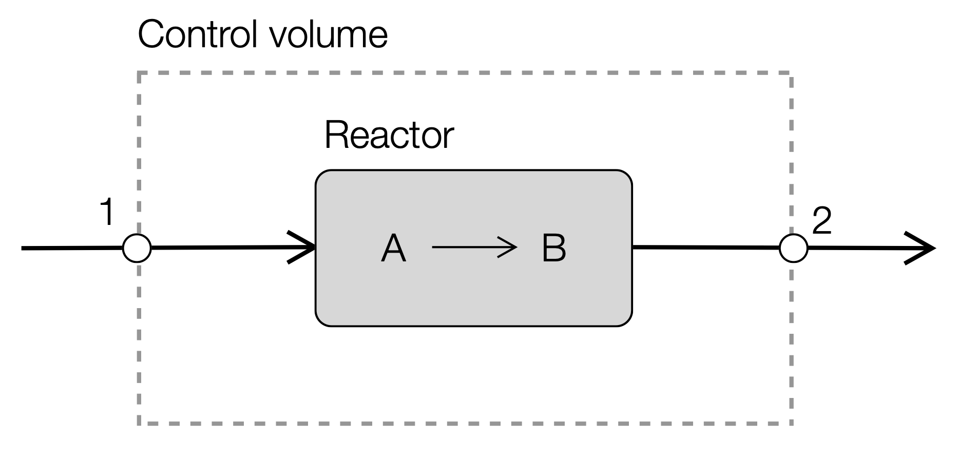
../_images/Fig-Reactor-Schematic.png — Fig. 11 Schematic of an open, well-mixed chemical reactor with a single input and output stream.#

The species set in this case is $\mathcal{M}=\left\{A,B\right\}$ and the stream set $\mathcal{S}=\left\{s_{1},s_{2}\right\}$, and there is a single chemical reaction; let $A$ be species 1 and $B$ be species 2. Definition 9 tells us that we’ll have a system of equations of the form (at steady-state):

\[\begin{split} \begin{eqnarray} \dot{n}_{A,1} - \dot{n}_{A,2} - \dot{\epsilon}_{1} & = & 0 \\ \dot{n}_{B,1} - \dot{n}_{B,2} + \dot{\epsilon}_{1} & = & 0 \\ \end{eqnarray} \end{split}\]

However, this steady-state system of mole balances can be rewritten in a more compact (and general) form:

(15)#\[\mathbf{N}\cdot\mathbf{d} + \mathbf{S}\cdot\dot{\mathbf{\epsilon}} = \mathbf{0}\]

The boldface capital letters denote matrices, while small letters denote vectors. In this particular case, $\mathbf{N}$ denotes the species flow matrix:

(16)#\[\begin{split}\mathbf{N} = \begin{bmatrix} \dot{n}_{11} & \dot{n}_{12} \\ \dot{n}_{21} & \dot{n}_{22} \\ \end{bmatrix}\end{split}\]

and $\mathbf{S}$ denotes the stoichiometric matrix:

(17)#\[\begin{split}\mathbf{S} = \begin{bmatrix} -1 \\ 1 \\ \end{bmatrix}\end{split}\]

while $\mathbf{d} = \left(1, -1\right)^{T}$ and $\dot{\mathbf{\epsilon}} = \dot{\epsilon}_{1}$. The superscript $\star^{T}$ denotes the transpose operation (turns a row into a column, or vice-versa). As it turns out, Eqn. (15) is a particular instance of a general system of equations that can be written in matrix-vector form (Definition 10):

Definition 10 (General open species mole balances)

The steady-state open species mole balances for a well-mixed system with species set $\mathcal{M}$, reaction set $\mathcal{R}$, and stream set $\mathcal{S}$ is described by:

\[\dot{\mathbf{N}}\cdot{\mathbf{d}} + \mathbf{S}\cdot\dot{\mathbf{\epsilon}} = \mathbf{0}\]

The matrix $\dot{\mathbf{N}}\in\mathbb{R}^{\mathcal{M}\times\mathcal{S}}$ is the species flow matrix, $\mathbf{d}\in\mathbb{R}^{\mathcal{S}\times{1}}$ is the stream direction vector, $\mathbf{S}\in\mathbb{R}^{\mathcal{M}\times\mathcal{R}}$ is the stoichiometric matrix, and $\dot{\mathbf{\epsilon}}\in\mathbb{R}^{\mathcal{R}\times{1}}$ is the open reaction extent vector. The open species mole balances can also be written in index form as:

\[\sum_{s\in\mathcal{S}}d_{s}\dot{n}_{is} + \sum_{r\in\mathcal{R}}\sigma_{ir}\dot{\epsilon}_{r} = 0\qquad{i=1,2,\dots,\mathcal{M}}\]

where $\dot{n}_{is}$ is the mole flow rate of species $i$ in stream $s$, $d_{s}$ is the direction of stream $s$, $\sigma_{ir}$ is the stoichiometric coefficient for species $i$ in reaction $r$, and $\dot{\epsilon}_{r}$ is the open extent of reaction $r$.

Matrices and vectors naturally arise in simple chemical engineering systems like the one shown in Fig. 11 Let’s dig deeper into their definition, structure, and operations.

Matrices and Vectors#

Matrices are two- (or more) dimensional rectangular arrays of numbers, widgets, etc. that consist of $m$ rows and $n$ columns:

\[\begin{split}\mathbf{A} = \begin{pmatrix} a_{1,1} & a_{1,2} & \cdots & a_{1,n} \\ a_{2,1} & a_{2,2} & \cdots & a_{2,n} \\ \vdots & \vdots & \ddots & \vdots \\ a_{m,1} & a_{m,2} & \cdots & a_{m,n} \end{pmatrix}\end{split}\]

The quantity $a_{ij}\in\mathbf{A}$ denotes an element of the matrix $\mathbf{A}$, where $a_{ij}$ lives on the $i$th row and $j$th column of $\mathbf{A}$. By convention, the row index is always the first subscript, while the column index is always listed second. Matrices can have different shapes (Observation 1):

Observation 1 (Matrix shape)

Let the matrix $\mathbf{A}$ be an $m\times{n}$ array. Then, the matrix $\mathbf{A}$ is called:

Square: If $m=n$, the matrix is called a square matrix; square matrices have some unique properties (as we shall see later).
Overdetermined: If $m>n$, the matrix is called an overdetermined matrix; overdetermined matrices have more rows than columns.
Underdetermined: If $m<n$, the matrix is called an underdetermined matrix; underdetermined matrices have more columns than rows.

Vectors are a special type of one-dimensional matrix where elements are arranged as a single row or column. For example, a $m\times{1}$ column vector $\mathbf{a}$ is given by:

\[\begin{split}\mathbf{a} = \begin{pmatrix} a_{1} \\ a_{2} \\ \vdots \\ a_{m} \end{pmatrix}\end{split}\]

while a ${1}\times{n}$ dimensional row vector $\mathbf{a}$ is given by:

\[\mathbf{a} = \begin{pmatrix} a_{1} & a_{2} & \cdots & a_{n} \end{pmatrix}\]

Just like numbers, vectors and matrices can participate in mathematical operations, such as addition, subtraction, and multiplication, with some small differences. However, before we explore the mathematical operations of matrices and vectors, we’ll discuss a few special matrices.

Remark 4 (Restriction to real numbers)

While the matrix $\mathbf{A}$ or vector $\mathbf{v}$ can theoretically hold any objects, e.g., strings, dictionaries, or trees, etc., in this section, we’ll only consider numbers and particular real numbers. Thus, we’ll assume all matrices are $\mathbf{A}\in\mathbb{R}^{n\times{m}}$ and vectors $\mathbf{v}\in\mathbb{R}^{n}$; no complex numbers will be considered.

Special matrices and matrix properties#

Special matrices have specific properties or characteristics that make them useful in certain mathematical operations or applications. Some examples of special matrices include:

Diagonal and identity matrices: A diagonal matrix is a square matrix in which all entries outside the main diagonal are zero. The unique diagonal matrix with 1 on the diagonal and 0 everywhere else is called the Identity matrix and is often denoted by the symbol $\mathbf{I}$.
Triangular matrices: Triangular matrices are square arrays with zero entries below or above the main diagonal. A square matrix is called lower triangular if all the entries above the main diagonal are zero. Similarly, a square matrix is called upper triangular if all the entries below the main diagonal are zero.
Orthogonal matrices: Orthogonal matrices are square matrices whose rows and columns are mutually orthogonal and have unit lengths.

Trace, Determinant, LU decomposition, and Rank#

Trace. The trace of a square matrix is the sum of the diagonal elements (Definition 11):

Definition 11 (Trace)

The trace of a square matrix is defined as the sum of its diagonal elements. Consider an $n\times{n}$ square matrix $\mathbf{A}\in\mathbb{R}^{n\times{n}}$, where $a_{ij}$ denotes the element on row $i$ and column $j$ of the matrix $\mathbf{A}$. Then, the trace, denoted as $\text{tr}\left(\mathbf{A}\right)$, is given by:

(18)#\[\text{tr}\left(\mathbf{A}\right) = \sum_{i=1}^{n}a_{ii}\]

In Julia, the trace function is encoded in the LinearAlgebra package included with the Julia distribution. However, the LinearAlgebra package is not loaded by default (you’ll need to issue the using LinearAlgebra command to access its functions):

# load the LinearAlgebra package
using LinearAlgebra

# Define array
A = [1 2 ; 3 4]; # the semicolon forces a newline 

# compute the trace store in the variable value
value = tr(A);

# What is the tr(A)
println("The trace of the matrix tr(A) = $(value)")

The trace of the matrix tr(A) = 5

NumPy also has a trace function if you are doing linear algebra calculations in Python. The determinant of a matrix is a scalar value that can be computed from a square matrix (Definition 12):

Definition 12 (Leibniz determinant formula)

The Leibniz determinant formula involves summing the products of elements in a square matrix, each taken from a different row and column, with a sign factor that alternates between positive and negative.

Let $\mathbf{A}\in\mathbb{R}^{n\times{n}}$ and $a_{ij}\in\mathbf{A}$ be the entry of row $i$ and column $j$ of $\mathbf{A}$. Then, the determinant $\det\left(\mathbf{A}\right)$ is given by:

(19)#\[\det\left(\mathbf{A}\right) = \sum_{\sigma\in{S_{n}}}\text{sign}\left(\sigma\right)\prod_{i=1}^{n}a_{i\sigma_{i}}\]

where $S_{n}$ denotes the Symmetry group of dimension $n$, i.e., the set of all possible permutations of the set ${1,2,\dots,n}$, the quantity $\text{sign}\left(\sigma\right)$ equals +1 if the permutation can be obtained with an even number of exchanges; otherwise -1. Finally, $a_{i\sigma_{i}}$ denotes the entry of the matrix $\mathbf{A}$ on row $i$, and column $\sigma_{i}$.

Determinants can be used to determine whether a system of linear equations has a solution, but they also have other applications. However, the Leibniz determinant shown in Definition 12 can be computationally expensive for large matrices since the number of permutations grows factorially with the matrix size. However, it provides a theoretical basis for understanding the determinant and can be helpful for small matrices or conceptual purposes. In Julia, the determinant function is encoded in the LinearAlgebra package included with the Julia distribution. However, the LinearAlgebra package is not loaded by default (you’ll need to issue the using LinearAlgebra command to access its functions):

# load the LinearAlgebra package
using LinearAlgebra

# Define array
A = [1 2 ; 3 4]; # the semicolon forces a newline 

# compute the determinant, and store in the variable value
value = det(A);

# What is the det(A)
println("The determinant of the matrix det(A) = $(value)")

The determinant of the matrix det(A) = -2.0

Although the determinant of a general square matrix is expensive to calculate, determinants of triangular matrices are easy to compute:

Observation 2 (Determinant triangular matrix)

The determinant of a triangular matrix is equal to the product of its diagonal elements. This is true for both upper triangular $\mathbf{U}$ and lower $\mathbf{L}$ triangular matrices. For example, the determinant of the upper triangular $n\times{n}$ matrix $\mathbf{U}$ is equal to:

\[\det\left(\mathbf{U}\right) = \prod_{i=1}^{n}u_{ii}\]

A similar expression could be written for a lower triangular matrix $\mathbf{L}$.

# load the LinearAlgebra package
using LinearAlgebra

# Define array
A = [1 0 ; 2 3]; # the semicolon forces a newline 

# compute the determinant, and store in the variable value
value = det(A);

# What is the det(A)
println("The determinant of the matrix det(A) = $(value)")

The determinant of the matrix det(A) = 3.0

LU decomposition. LU decomposition, also known as LU factorization, is a method of decomposing a square matrix $\mathbf{A}\in\mathbb{R}^{n\times{n}}$ into the product of a permutation matrix $\mathbf{P}$, and lower and upper triangular matrices $\mathbf{L}$ and $\mathbf{U}$, respectively, such that $\mathbf{A} = \mathbf{P}\mathbf{L}\mathbf{U}$. LU decomposition is a widely used numerical linear algebra technique with many applications. For example, the LU decomposition simplifies the computation of determinants (Definition 13):

Definition 13 (LU decomposition)

Let the $\mathbf{A}\in\mathbb{R}^{n\times{n}}$ be LU factoriable, such that $\mathbf{A} = \mathbf{P}\mathbf{L}\mathbf{U}$. Then, the determinant $\det\left(\mathbf{A}\right)$ is given by:

(20)#\[\det\left(\mathbf{A}\right) = \det\left(\mathbf{P}\right)\cdot\det\left(\mathbf{L}\right)\cdot\det\left(\mathbf{U}\right)\]

In Julia, the LU factorization is encoded in the LinearAlgebra package included with the Julia standard library:

# load the LinearAlgebra package
using LinearAlgebra

# Define array
A = [1 2 ; 3 4]; # the semicolon forces a newline 

# compute the determinant and store it in the variable value
F = lu(A);
L = F.L
U = F.U
P = F.P

# Test -
AT = P*L*U

2×2 Matrix{Float64}:
 1.0  2.0
 3.0  4.0

Rank. Finally, the rank of a matrix is a measure of the number of linearly independent rows or columns (Definition 14):

Definition 14 (Rank)

The rank of a matrix r of a $m\times{n}$ matrix $\mathbf{A}$ is always less than or equal to the minimum of its number of rows and columns:

(21)#\[r\leq\min\left(m,n\right)\]

Rank can also be considered a measure of the unique information in a matrix; if there is redundant information (rows or columns that are not linearly independent), a matrix will have less than full rank.

# load the LinearAlgebra package
using LinearAlgebra

# Define array
A = [1 2 ; 3 4]; # the semicolon forces a newline 

# compute the rank, store in the variable value
value = rank(A);

# What is the rank(A)
println("The rank of the matrix rank(A) = $(value)")

The rank of the matrix rank(A) = 2

Mathematical matrix and vector operations#

Matrix and vector operations are mathematical procedures for adding, subtracting, and multiplying matrices and vectors. They are similar in some ways to scalar numbers, but they have some crucial differences and one important caveat: they must be compatible.

Many (if not all) modern programming languages implement a version of the Basic Linear Algebra Subprograms (BLAS) library. BLAS is a low-level library that efficiently implements basic linear algebra operations, such as vector and matrix multiplication, matrix-vector multiplication, and solving linear systems of equations. The library is designed to provide high-performance implementations of these routines that can be used as building blocks for more complex algorithms. However, while you will not have to implement most matrix and vector operations on your own, it is still helpful to understand these operations and how broadly they work.

Addition and subtraction#

Compatible matrices and vectors can be added and subtracted just like scalar quantities. The addition (or subtraction) operations for matrices or vectors are done element-wise. Thus, if these objects have a different number of elements, then addition and subtraction operations don’t make sense.

Definition 15 (Vector addition)

Suppose we have two vectors $\mathbf{a}\in\mathbb{R}^{m}$ and $\mathbf{b}\in\mathbb{R}^{m}$. The sum of these vectors $\mathbf{y} = \mathbf{a} + \mathbf{b}$ is the vector $\mathbf{y}\in\mathbb{R}^{m}$ given by:

(22)#\[y_{i} = a_{i} + b_{i}\qquad{i=1,\dots,m}\]

Compatibility: The vectors $\mathbf{a}$ and $\mathbf{b}$ are compatible if they have the same number of elements.

Vector addition is straightforward to implement (Algorithm 4):

Algorithm 4 (Naive vector addition)

Inputs Compatible vectors $\mathbf{a}$ and $\mathbf{b}$

Outputs Vector sum $\mathbf{y}$

Initialize

set $n\leftarrow\text{length}(\mathbf{a})$
set $\mathbf{y}\leftarrow\text{zeros}(n)$

Main

for $i\in{1,\dots,n}$
1. $y_{i}\leftarrow~a_{i} + b_{i}$

Return sum vector $\mathbf{y}$

Is the naive approach the best?#

Algorithm 4 may not be the best way to implement vector (or matrix) addition or subtraction operations. Many modern programming languages and libraries, e.g., the Numpy library in Python or Julia, support vectorization, i.e., special operators that encode element-wise addition, subtraction or other types of element-wise operations without the need to write for loops. In Julia, you can use the vectorized .+ operator for element-wise addition, while element-wise subtraction can be encoded with the .- operator. Vectorized code typically executes faster than naive implementations such as Algorithm 4 because the vectorization takes advantage of advanced techniques to improve performance.

Vectorized operations in NumPy. NumPy is a Python scientific computing package. It is a Python library that provides multidimensional array objects and routines for fast operations on arrays.
Vectorized operations in Julia are included in the standard library. The standard library already defines common operators such as addition .+, subtraction .-, multiplication .*, and power .^. However, the broadcasting paradigm allows you to write your own vectorized operations.

Multiplication operations#

The most straightforward multiplication operation is between a scalar and a vector (or matrix). Multiplying a vector (or a matrix) by a scalar constant is done element-wise (Definition 16):

Definition 16 (Scalar multiplication of a matrix or vector)

Vector: Suppose we have a vector $\mathbf{v}\in\mathbb{R}^{n}$ and a real scalar constant $c\in\mathbb{R}$. Then the scalar product, denoted by $\mathbf{y} = c\mathbf{v}$, is given by:

\[y_{i} = cv_{i}\qquad{i=1,2,\dots,n}\]

where $y_{i}$ and $v_{i}$ denote the ith component of the product vector $\mathbf{y}\in\mathbb{R}^{n}$, and the input vector $\mathbf{v}\in\mathbb{R}^{n}$.

Matrix: Likewise, suppose we have the matrix $\mathbf{X}\in\mathbb{R}^{m\times{n}}$ and a real scalar constant $c\in\mathbb{R}$. Then, the scalar product, denoted by $\mathbf{Y} = c\mathbf{X}$, is given by:

\[y_{ij} = cx_{ij}\qquad{i=1,2,\dots,m,~j=1,2,\dots,n}\]

where $y_{ij}$ and $x_{ij}$ denote components of the product matrix $\mathbf{Y}\in\mathbb{R}^{m\times{n}}$, and the input matrix $\mathbf{X}\in\mathbb{R}^{m\times{n}}$, respectively.

Vector-vector operations#

Inner product: Two compatible vectors $\mathbf{a}$ and $\mathbf{b}$ can be multiplied together to produce a scalar in an operation called an inner product operation (Definition 17):

Definition 17 (Inner product)

Let $\mathbf{a}\in\mathbb{R}^{m\times{1}}$ and $\mathbf{b}\in\mathbb{R}^{m\times{1}}$. Then, the vector-vector inner product is given by:

(23)#\[y = \mathbf{a}^{T}\mathbf{b}\]

where $\mathbf{a}^{T}$ denotes the transpose of the vector $\mathbf{a}$ and the scalar $y$ equals:

(24)#\[y = \sum_{i=1}^{m}a_{i}b_{i}\]

Compatibility: This operation is possible if the vectors $\mathbf{a}$ and $\mathbf{b}$ have the same number of elements.

Outer product: Suppose you have an $m\times{1}$ vector $\mathbf{a}$, and an $n\times{1}$ vector $\mathbf{b}$. The vectors $\mathbf{a}$ and $\mathbf{b}$ can be multiplied together to form a $m\times{n}$ matrix through an outer product operation (Definition 18):

Definition 18 (Outer product)

Let $\mathbf{a}\in\mathbb{R}^{m\times{1}}$ and $\mathbf{b}\in\mathbb{R}^{n\times{1}}$. Then, the vector-vector outer product given by:

(25)#\[\mathbf{Y} = \mathbf{a}\otimes\mathbf{b}\]

produces the matrix $\mathbf{Y}\in\mathbb{R}^{m\times{n}}$ with elements:

(26)#\[y_{ij} = a_{i}b_{j}\qquad{i=1,2,\dots,m~\text{and}~j=1,2,\dots,n}\]

The outer product operation is equivalent to $\mathbf{Y} = \mathbf{a}\mathbf{b}^{T}$.

Compatibility: This operation is possible if the vectors $\mathbf{a}$ and $\mathbf{b}$ have the same number of elements.

Right multiplication of a matrix by a vector#

A common operation is right matrix-vector multiplication of a matrix $\mathbf{A}$ by a vector $\mathbf{x}$. If the matrix $\mathbf{A}$ and the vector $\mathbf{x}$ are compatible, right matrix-vector multiplication will produce a vector with the same number of rows as the original matrix $\mathbf{A}$ (Definition 19):

Definition 19 (Right matrix-vector multiplication)

Let $\mathbf{A}\in\mathbb{R}^{m\times{n}}$ and $\mathbf{x}\in\mathbb{R}^{n\times{1}}$. Then, the right matrix-vector product is given by:

\[\mathbf{y} = \mathbf{A}\mathbf{x}\]

generates the $\mathbf{y}\in\mathbb{R}^{m\times{1}}$ vector where the $i$th element is given by:

\[y_{i} = \sum_{j=1}^{n}a_{ij}x_{j}\qquad{i=1,2,\cdots,m}\]

Compatibility: This operation is possible if the number of columns of the matrix $\mathbf{A}$ equals the number of rows of the vector $\mathbf{x}$.

The right multiplication operation can be represented graphically as a series of scalar$\times$vector multiplication and vector-vector summation operations (Fig. 12):

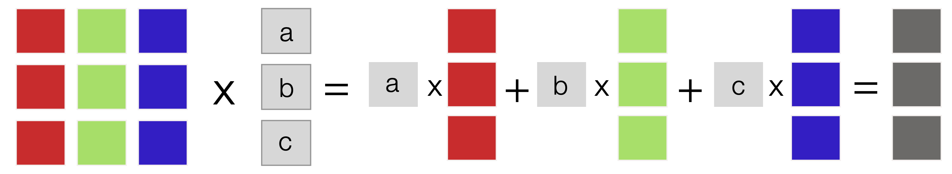
../_images/Fig-Ab-Multiplication.png — Fig. 12 Schematic of the right matrix-vector product. The right product, which produces a column vector with the same number of rows as the matrix, can be modeled as a series of scalar$\times$vector multiplication and vector-vector summation operations.#

A pseudo code implementation of Definition 19 is given in Algorithm 5:

Algorithm 5 (Naive right multiplication of a matrix by a vector)

Inputs: Matrix $\mathbf{A}\in\mathbb{R}^{m\times{n}}$ and vector $\mathbf{x}\in\mathbb{R}^{n\times{1}}$

Outputs: Product vector $\mathbf{y}\in\mathbb{R}^{m\times{1}}$.

Initialize

set $(m, n)\leftarrow\text{size}(\mathbf{A})$
initialize $\mathbf{y}\leftarrow\text{zeros}(m)$

Main

for $i\in{1,\dots,m}$:
1. for $j\in{1,\dots,n}$:
  1. $y_{i}~\leftarrow y_{i} + a_{ij}\times{x_{j}}$

Return vector $\mathbf{y}$

Left multiplication of a matrix by a vector#

We could also consider the left multiplication of a matrix by a vector. Suppose $\mathbf{A}$ is an $m\times{n}$ matrix, and $\mathbf{x}$ is a $m\times{1}$ vector, then the left matrix-vector product is a row vector (Definition 20):

Definition 20 (Left matrix-vector product)

Let $\mathbf{A}\in\mathbb{R}^{m\times{n}}$ and $\mathbf{x}\in\mathbb{R}^{m\times{1}}$. Then, the left matrix-vector product:

(27)#\[\mathbf{y} = \mathbf{x}^{T}\mathbf{A}\]

produces the vector $\mathbf{y}\in\mathbb{R}^{1\times{n}}$ such that:

(28)#\[y_{i} = \sum_{j=1}^{m}a_{ji}x_{j}\qquad{i=1,2,\dots,n}\]

where $\mathbf{x}^{T}$ denotes the transpose of the vector $\mathbf{x}$.

Compatibility: This operation is possible if the number of rows of the matrix $\mathbf{A}$ equals the number of columns of the transpose of the vector $\mathbf{x}$.

The left multiplication operation can be represented graphically as a series of scalar$\times$vector multiplication and vector-vector summation operations (Fig. 13):

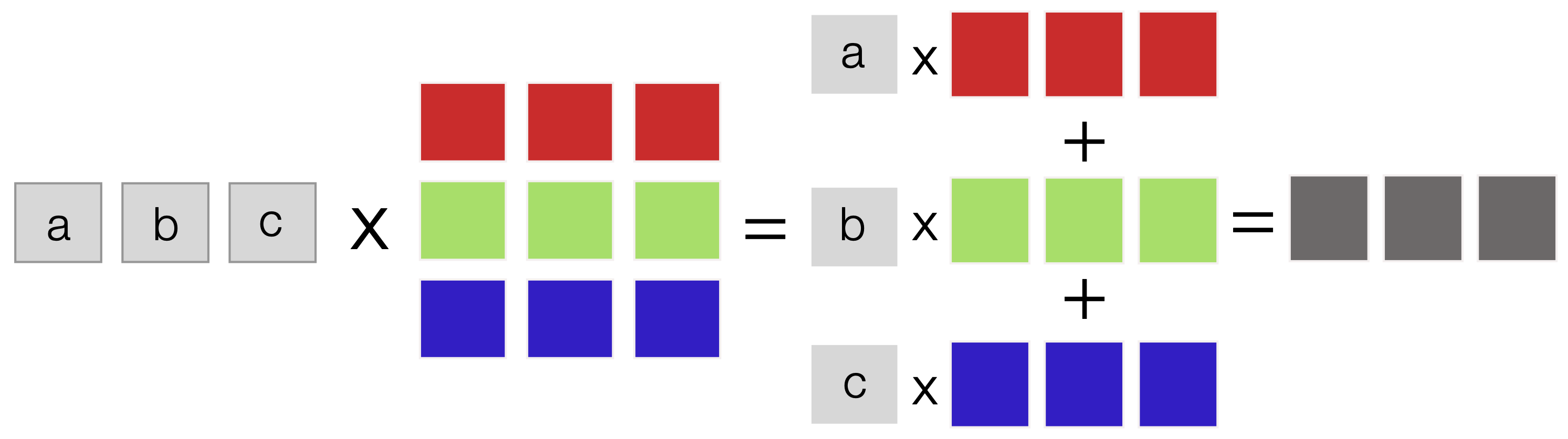
../_images/Fig-bA-Left-Multiplication.png — Fig. 13 Schematic of the left matrix-vector product. The left product, which produces a row vector with the same number of columns as the matrix, can be modeled as a series of scalar$\times$vector multiplication and vector-vector summation operations.#

A psuedo code implemetation of Definition 20 is given in Algorithm 6:

Algorithm 6 (Naive left multiplication of a matrix by a vector)

Inputs: Matrix $\mathbf{A}\in\mathbb{R}^{m\times{n}}$ and vector $\mathbf{x}\in\mathbb{R}^{m\times{1}}$

Outputs: Product vector $\mathbf{y}\in\mathbb{R}^{1\times{n}}$.

Initialize

set $(m, n)\leftarrow\text{size}(\mathbf{A})$
initialize $\mathbf{y}\leftarrow\text{zeros}(n)$

Main

for $i\in{1,\dots,n}$:
1. for $j\in{1,\dots,m}$:
  1. $y_{i}~\leftarrow y_{i} + a_{ji}\times{x_{j}}$

Return vector $\mathbf{y}$

Matrix-Matrix products#

Many of the important uses of matrices in engineering practice depend upon the definition of matrix multiplication (Definition 21):

Definition 21 (Matrix-matrix product)

Let $\mathbf{A}\in\mathbb{R}^{m\times{n}}$ and $\mathbf{B}\in\mathbb{R}^{n\times{p}}$. The matrix-matrix product $\mathbf{C} = \mathbf{A}\times\mathbf{B}$ produces the matrix $\mathbf{C}\in\mathbb{R}^{m\times{p}}$ with elements:

(29)#\[c_{ij} = \sum_{k=1}^{n}a_{ik}b_{kj}\qquad{i=1,2,\cdots,m~\text{and}~j=1,2,\cdots,p}\]

Compatibility: The matrices $\mathbf{A}\in\mathbb{R}^{m\times{n}}$ and $\mathbf{B}\in\mathbb{R}^{n\times{p}}$ are compatible if the number of columns of $\mathbf{A}\in\mathbb{R}^{m\times{n}}$ equals the number of rows of $\mathbf{B}\in\mathbb{R}^{n\times{p}}$. Otherwise, the matrices are incompatible and cannot be multiplied.

The matrix-matrix multiplication operation can be represented graphically as a series of right matrix-vector products (Fig. 14):

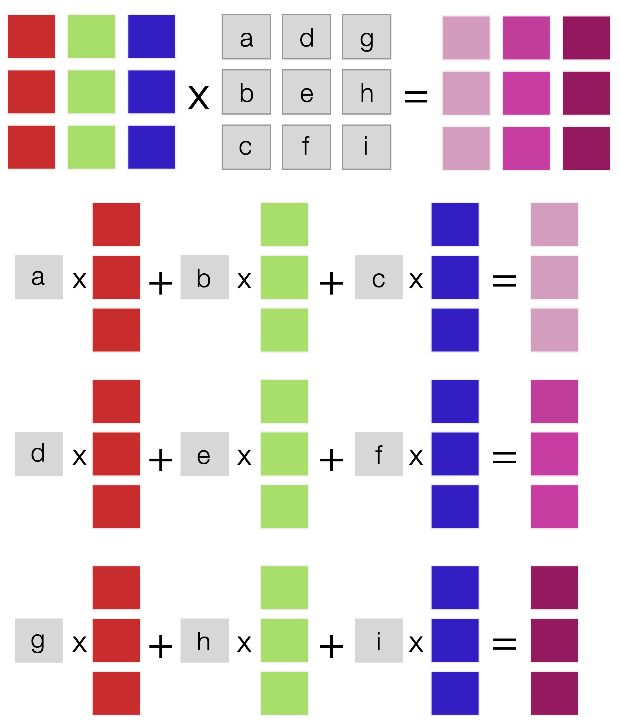
../_images/Fig-AB-Matrix-Matrix-Multiplication.png — Fig. 14 Schematic of matrix-matrix multiplication. This operation produces a matrix product and can be modeled as a series of right matrix-vector products.#

A pseudo-code implementation of Definition 21 is given in Algorithm 7:

Algorithm 7 (Naive Matrix $\times$ Matrix multiplication)

Inputs Matrix $\mathbf{A}\in\mathbb{R}^{m\times{n}}$, and matrix $\mathbf{B}\in\mathbb{R}^{n\times{p}}$

Outputs Product matrix $\mathbf{C}\in\mathbb{R}^{m\times{p}}$.

Initialize

initialize $(m, n)\leftarrow\text{size}(\mathbf{A})$
initialize $(n, p)\leftarrow\text{size}(\mathbf{B})$
initialize matrix $\mathbf{C}\leftarrow\text{zeros}(m, p)$

Main

for $i\in{1,\dots, m}$
1. for $j\in{1,\dots,p}$
  1. for $k\in{1,\dots,n}$
    1. $c_{ij}~\leftarrow~c_{ij} + a_{ik}\times{b_{kj}}$

Return matrix $\mathbf{C}$

Finally, matrix-matrix products have different properties compared with the product of two scalar numbers:

Non-commutativity: Matrix multiplication is typically not commutative, e.g., $\mathbf{A}\mathbf{B}\neq\mathbf{B}\mathbf{A}$.
Distributivity: Matrix products are distributive, i.e., $\mathbf{A}\left(\mathbf{B}+\mathbf{C}\right) = \mathbf{A}\mathbf{B}+\mathbf{A}\mathbf{C}$.
Associative: Matrix products are associative, i.e., $\mathbf{A}\left(\mathbf{B}\mathbf{C}\right) = \left(\mathbf{A}\mathbf{B}\right)\mathbf{C}$.
Transpose: The transpose of a matrix product is the product of transposes, i.e., $\left(\mathbf{A}\mathbf{B}\right)^{T} = \mathbf{B}^{T}\mathbf{A}^{T}$.

Linear algebraic equations#

Linear Algebraic Equations (LAEs) arise in many different engineering fields. In Chemical Engineering, these equations naturally arise from steady-state (or time-discretized) balances. Let’s start by asking a simple question: when does a solution exist to the generic system of LAEs of the form:

(30)#\[\mathbf{A}\mathbf{x} = \mathbf{b}\]

where $\mathbf{A}\in\mathbb{R}^{m\times{n}}$ is the system matrix, $\mathbf{x}\in\mathbb{R}^{n\times{1}}$ denotes a column vector of unknowns (what we want to solve for), and $\mathbf{b}\in\mathbb{R}^{m\times{1}}$ is the right-hand side vector:

Homogenous system: A homogeneous system of linear algebraic equations is a system in which the right-hand side vector $\mathbf{b}= \mathbf{0}$; every entry in the $\mathbf{b}$-vector is equal to zero. The solution set for a homogeneous system is a subspace in linear algebra called the kernel or nullpsace.
Non-homogeneous system: A non-homogeneous system of linear algebraic equations is a system in which at least one entry of the right-hand side vector $\mathbf{b}$ is non-zero.

Existence#

The existence of a solution to a system of linear equations depends on the right-hand side vector, the number of equations, and the number of variables in the system. For a homogeneous square system of linear equations, the trivial solution $\mathbf{x}=\mathbf{0}$ always exists. However, a homogeneous square system of linear algebraic equations with $n\times{n}$ system matrix $\mathbf{A}\in\mathbb{R}^{n\times{n}}$ and unknown vector $\mathbf{x}\in\mathbb{R}^{n\times{1}}$:

(31)#\[\mathbf{A}\mathbf{x} = \mathbf{0}\]

may have other solutions. There is an easy check to determine the existence of other solutions for a homogenous square system (Definition 22):

Definition 22 (Homogenous solution existence)

A $n\times{n}$ homogeneous system of linear algebraic equations will have non-trivial solutions if and only if the system matrix $\mathbf{A}\in\mathbb{R}^{n\times{n}}$ has a zero determinant:

(32)#\[\det\left(\mathbf{A}\right) = 0\]

The determinant condition is an easy theoretical test to check for the existence of solutions to a homogenous system of linear algebraic equations. Existence can also be checked by computing the rank: if a matrix is less than full rank, then $\det{\left(\mathbf{A}\right)}=0$.

Non-homogeneous square systems#

A non-homogeneous square system of linear algebraic equations with matrix $\mathbf{A}\in\mathbb{R}^{n\times{n}}$, unknown vector $\mathbf{x}\in\mathbb{R}^{n\times{1}}$ and the right-hand-side vector $\mathbf{b}\in\mathbb{R}^{n\times{1}}$:

(33)#\[\mathbf{A}\mathbf{x} = \mathbf{b}\]

will have a unique solution if there exists a matrix $\mathbf{A}^{-1}\in\mathbb{R}^{n\times{n}}$ such that:

(34)#\[\mathbf{x} = \mathbf{A}^{-1}\mathbf{b}\]

where the $\mathbf{A}^{-1}$ is called the inverse of the matrix $\mathbf{A}$ (Definition 23):

Definition 23 (Matrix inverse existence)

An $n\times{n}$ square matrix $\mathbf{A}\in\mathbb{R}^{n\times{n}}$ has an unique inverse $\mathbf{A}^{-1}$ such that:

(35)#\[\mathbf{A}^{-1}\mathbf{A} = \mathbf{A}\mathbf{A}^{-1} = \mathbf{I}\]

if $\det\left(\mathbf{A}\right)\neq{0}$. If an inverse exists, the matrix $\mathbf{A}$ is called non-singular; otherwise, $\mathbf{A}$ is singular.

In Julia, the matrix inverse can be calculated using the inv function. Similarly, the NumPy library for Python has a similar inv function.

Solutions approaches#

Several methods exist to find the solution of square systems of linear equations:

Gaussian elimination solves linear equations by using a sequence of operations to reduce the system to an upper triangular form and then back substitution to find the solution.
Iterative solution methods are another class of algorithms used to find approximate solutions for large and sparse linear systems of equations. These methods work by starting with an initial guess for the solution and then repeatedly updating the guess until it converges to the actual answer.

Gaussian elimination#

Gaussian elimination is an efficient method for solving large square systems of linear algebraic equations. Gaussian elimination is based on “eliminating” variables by adding or subtracting equations (rows) so that the coefficients of one variable are eliminated in subsequent equations. This allows us to solve the remaining variables individually until we have a solution for the entire system. Let’s start exploring this approach by looking at solving a triangular system of equations.

Triangular systems#

Let’s consider a non-singular $3\times{3}$ lower triangular system of equations:

(36)#\[\begin{split}\begin{pmatrix} l_{11} & 0 & 0 \\ l_{21} & l_{22} & 0 \\ l_{31} & l_{32} & l_{33} \end{pmatrix} \begin{pmatrix} x_{1} \\ x_{2} \\ x_{3} \end{pmatrix} = \begin{pmatrix} b_{1} \\ b_{2} \\ b_{3} \end{pmatrix}\end{split}\]

Since the matrix is non-singular, the diagonal elements $l_{ii},~i=1,2,3$ are non-zero. This allows us to take advantage of the triangular structure to solve for the unknown $x_{i}$ values:

\[\begin{split} \begin{eqnarray} x_{1} & = & b_{1}/l_{11} \\ x_{2} & = & \left(b_{2} - l_{21}x_{1}\right) / l_{22} \\ x_{3} & = & \left(b_{3} - l_{31}x_{1} - l_{32}x_{2}\right) / l_{33} \end{eqnarray} \end{split}\]

This idea, called forward substitution, can be extended to any $n\times{n}$ non-singular lower triangular system (Definition 24):

Definition 24 (Forward substitution)

Suppose we have an $n\times{n}$ system ($n\geq{2}$) of equations which is lower triangular and non-singular of the form:

(37)#\[\mathbf{L}\mathbf{x} = \mathbf{b}\]

Then, the solution of Eqn. (37) is given by:

\[\begin{split} \begin{eqnarray} x_{1} & = & \frac{b_{1}}{l_{11}} \\ x_{i} & = & \frac{1}{l_{ii}}\left(b_{i} - \sum_{j=1}^{i-1}l_{ij}x_{j}\right)\qquad{i=2,\dots,n} \end{eqnarray} \end{split}\]

where $l_{ii}\neq{0}$. The global operation count for this approach is $n^{2}$ floating point operations (flops).

Alternatively, we can take a similar approach with an upper triangular system, called backward substitution, to solve for unknow solution vector $\mathbf{x}$ (Definition 25):

Definition 25 (Backward substitution)

Suppose we have an $n\times{n}$ system ($n\geq{2}$) of equations which is upper triangular and non-singular of the form:

(38)#\[\mathbf{U}\mathbf{x} = \mathbf{b}\]

Then, the solution of Eqn. (38) is given by:

\[\begin{split} \begin{eqnarray} x_{n} & = & \frac{b_{n}}{u_{nn}} \\ x_{i} & = & \frac{1}{u_{ii}}\left(b_{i} - \sum_{j=i+1}^{n}u_{ij}x_{j}\right)\qquad{i=n-1,\dots,1} \end{eqnarray} \end{split}\]

where $u_{ii}\neq{0}$. The global operation count for this approach is $n^{2}$ floating point operations (flops).

A substitution approach quickly solves a lower or upper triangular system. However, upper (or lower) triangular systems rarely arise naturally in applications. So why do we care about triangular systems?

Row reduction approaches#

Converting a matrix $\mathbf{A}$ to an upper triangular form involves performing a sequence of elementary row operations to transform the matrix into a form where all entries below the main diagonal are zero. This is typically done by row swapping, scaling, and adding rows. The goal is to create a matrix where each row’s leading coefficient (the first non-zero element) is 1, and all the other entries in that column are 0. This is achieved by using the leading coefficient of one row to eliminate the corresponding entries in the different rows.

Let’s walk through a simple example to illustrate the steps involved with row reduction; consider the solution of the 3$\times$3 system:

(39)#\[\begin{split}\begin{bmatrix} 2 & -1 & 0 \\ -1 & 2 & -1 \\ 0 & -1 & 2 \end{bmatrix} \begin{pmatrix} x_{1} \\ x_{2} \\ x_{3} \end{pmatrix} = \begin{pmatrix} 0 \\ 1 \\ 0 \end{pmatrix}\end{split}\]

Step 1: Form the augmented matrix $\bar{\mathbf{A}}$ which is defined as the matrix $\mathbf{A}$ with the right-hand-side vector $\mathbf{b}$ appended as the last column:

(40)#\[\begin{split}\bar{\mathbf{A}} = \begin{bmatrix} 2 & -1 & 0 &\bigm| & 0 \\ -1 & 2 & -1 &\bigm| & 1 \\ 0 & -1 & 2 &\bigm| & 0 \end{bmatrix}\end{split}\]

Step 2: Perform row operations to reduce the augmented matrix $\bar{\mathbf{A}}$ to the upper triangular row echelon form. We can perform row operations:

Swapping: We can interchange the order of the rows to get zeros below the main diagonal.
Scaling: If the first nonzero entry of row $R_{i}$ is $\lambda$, we can convert to $1$ through the operation: $R_{i}\leftarrow{1/\lambda}R_{i}$
Addition and subtraction: For any nonzero entry below the top one, use an elementary row operation to change it to zero. If two rows $R_{i}$ and $R_{j}$ have nonzero entries in column $k$, we can transform the (j,k) entry into a zero using $R_{j}\leftarrow{R}_{j} - (a_{jk}/a_{ik})R_{i}$.

In Eqn (40), the first row and column entry are non-zero, and interchanging rows does not improve our progress. However, the leading non-zero coefficient is not 1; thus, let’s use a scaling row operation:

(41)#\[\begin{split}\bar{\mathbf{A}} = \begin{bmatrix} 2 & -1 & 0 &\bigm| & 0 \\ -1 & 2 & -1 &\bigm| & 1 \\ 0 & -1 & 2 &\bigm| & 0 \end{bmatrix} \stackrel{R_{1}\leftarrow(1/2)R_{1}}{\longrightarrow} \begin{bmatrix} 1 & -0.5 & 0 &\bigm| & 0 \\ -1 & 2 & -1 &\bigm| & 1 \\ 0 & -1 & 2 &\bigm| & 0 \end{bmatrix}\end{split}\]

We now eliminate the coefficient below the top row; in this case $i=1$, $j=1$ and $k=1$ which gives the operation: $R_{2}\leftarrow{R}_{2} + R_{1}$:

(42)#\[\begin{split}\begin{bmatrix} 1 & -0.5 & 0 &\bigm| & 0 \\ -1 & 2 & -1 &\bigm| & 1 \\ 0 & -1 & 2 &\bigm| & 0 \end{bmatrix} \stackrel{R_{2}\leftarrow{R_{2}+R_{1}}}{\longrightarrow} \begin{bmatrix} 1 & -0.5 & 0 &\bigm| & 0 \\ 0 & 1.5 & -1 &\bigm| & 1 \\ 0 & -1 & 2 &\bigm| & 0 \end{bmatrix}\end{split}\]

The leading coefficient of row 3 was already zero; thus, we have completed the row reduction operations for row 1. Moving to row 2, the first non-zero coefficient is in column 2. Scale row 2, and then subtract from row 3, etc. While the logic underlying the row reduction of the matrix $\mathbf{A}$ to the upper triangular row-echelon form $\mathbf{U}$ seems simple, the implementation of a general, efficient row reduction function can be complicated; let’s develop a naive implementation of a row reduction procedure (Algorithm 8):

Algorithm 8 (Naive Row Reduction)

Input: Matrix $\mathbf{A}$, the vector $\mathbf{b}$

Output: solution $\hat{\mathbf{x}}$

Initialize:

set $(n,m)\leftarrow\text{size}(\mathbf{A})$
set $\bar{\mathbf{A}}\leftarrow\text{augment}(\mathbf{A},\mathbf{b})$

Main

for $i\in{1}\dots{n-1}$
1. set $\text{pivot}\leftarrow{a_{ii}}$
2. set $\text{pivotRow}\leftarrow{i}$
3. for $j\in{i+1}\dots{n}$
  1. if $\text{abs}(\bar{a}_{ji}) > \text{abs}(\text{pivot})$
    1. set $\text{pivot}\leftarrow\bar{a}_{ji}$
    2. set $\text{pivotRow}\leftarrow{j}$
4. set $\bar{\mathbf{A}}\leftarrow\text{swap}(\bar{\mathbf{A}},i,\text{pivotRow})$
5. for $j\in{i+1}\dots{n}$
  1. set $\text{factor}\leftarrow{a_{ji}}/\text{pivot}$
  2. for $k\in{1,\dots,m}$
    1. set $a_{jk}\leftarrow{a_{jk}} - \text{factor}\times{a_{ik}}$

Return $\text{row reduced}~\bar{\mathbf{A}}$

Step 3: Solve for the unknown values $x_{1},\dots,x_{n}$ using back substitution:

(43)#\[\begin{split}\begin{bmatrix} 1 & -0.5 & 0 &\bigm| & 0 \\ 0 & 1 & -0.66 &\bigm| & 0.66 \\ 0 & 0 & 1 &\bigm| & 0.49 \end{bmatrix}\end{split}\]

This system in Eqn. (43) is in row reduced form; thus, it can now be solved using back substitution. Based on the Definition 25, we implemented a back substitution routine Algorithm 9:

Algorithm 9 (Backward substituion)

Inputs Upper triangular matrix $\mathbf{U}$, column vector $\mathbf{b}$

Outputs solution vector $\mathbf{x}$

Initialize

set $n\leftarrow\text{nrows}\left(\mathbf{U}\right)$
set $\mathbf{x}\leftarrow\text{zeros}\left(n\right)$
set $x_n\leftarrow{b_n/u_{nn}}$

Main

for $i\in{n-1\dots,1}$
1. set $\text{sum}\leftarrow{0}$
2. for $j\in{i+1,\dots,n}$
  1. $\text{sum}\leftarrow\text{sum} + u_{ij}\times{x_{j}}$
3. $x_{i}\leftarrow\left(1/u_{ii}\right)\times\left(b_{i} - \text{sum}\right)$

Return solution vector $\mathbf{x}$

Now that we have row reduction and back substitution algorithms let’s look at a few examples. First, consider the solution of a square system of equations that arise from mole balance with a single first-order decay reaction (Example 19):

Example 19 (First-order decay)

Set up a system of linear algebraic equations whose solution describes the concentration as a function of time for a compound $A$ that undergoes first-order decay in a well-mixed batch reactor. The concentration balance for compound $A$ is given by:

(44)#\[\frac{dC_{A}}{dt} = -\kappa{C_{A}}\]

where $\kappa$ denotes the first-order rate constant governing the rate of decay (units: 1/time), and the initial condition is given by $C_{A,0}$. Let $C_{A,0} = 10~\text{mmol/L}$, $\kappa = 0.5~\text{hr}^{-1}$ and $h = 0.1$.

Solution: Let’s discretize the concentration balance using a forward finte difference approximation of the time derivatrive:

(45)#\[C_{A,j+1} = C_{A,j} - h\kappa{C_{A,j}}\]

where $h$ denotes the time step-size, and $C_{A,\star}$ denotes the concentration of $A$ at time-step $\star$. Starting with $j=0$, Eqn (45) can be used to construct a $T{\times}T$ matrix where each rows is a seperate time-step:

(46)#\[\begin{split}\begin{pmatrix} 1 & 0 & \dots & 0 \\ (\kappa{h} - 1) & 1 & \dots & 0 \\ \vdots & \vdots & \vdots & \vdots \\ 0 & \dots & (\kappa{h} - 1) & 1 \end{pmatrix} \begin{pmatrix} C_{A,1} \\ C_{A,2} \\ \vdots \\ C_{A,T} \end{pmatrix} = \begin{pmatrix} C_{A,0}\left(1-h\kappa\right) \\ 0 \\ \vdots \\ 0 \end{pmatrix}\end{split}\]

Iterative solution methods#

Iterative methods work by improving an initial guess of the solution until a desired level of accuracy is achieved. Commonly used iterative methods include Jacobi’s method and the Gauss-Seidel method.

At each iteration: an iterative method uses the current estimate of the solution to generate a new estimate closer to the actual answer. This process continues until the solution converges to a desired accuracy level, typically measured by a tolerance parameter. The basic strategy of an iterative method is shown in Observation 3:

Observation 3 (Basic iterative strategy)

Suppose we have a square system of linear algebraic equations:

\[\mathbf{A}\mathbf{x} = \mathbf{b}\]

where $\mathbf{A}\in\mathbb{R}^{n\times{n}}$ is the system matrix, $\mathbf{x}\in\mathbb{R}^{n\times{1}}$ is a vector of unknowns, and $\mathbf{b}\in\mathbb{R}^{n\times{1}}$ is the right-hand-side vector. Starting with equation $i$:

\[\sum_{j = 1}^{n}a_{ij}x_{j} = b_{i}\qquad{i=1,2,\cdots{n}}\]

we solve for an estimate of the ith unknown value $\hat{x}_{i}$:

\[\hat{x}_{i}=\frac{1}{a_{ii}}\bigl(b_{i}-\sum_{j=1,i}^{n}a_{ij}x_{j}\bigr)\qquad{i=1,2,\cdots{n}}\]

where $\sum_{j=1,i}^{n}$ does not include index $i$. What we do with the estimated value of $\hat{x}_{i}$ is the difference between Jacobi’s and Gauss-Seidel’s methods.

Iterative solution methods are used to solve large systems of linear equations where direct methods (such as Gaussian elimination) are impractical due to their computational cost.

Jacobi’s method#

Jacobi’s method batch updates the estimate of $x_{i}$ at the end of each iteration. Let the estimate of the value of $x_{i}$ at iteration k be $\hat{x}_{i,k}$. Then, the solution estimate at the next iteration $\hat{x}_{i,k+1}$ is given by:

(47)#\[\hat{x}_{i,k+1}=\frac{1}{a_{ii}}\bigl(b_{i}-\sum_{j=1,i}^{n}a_{ij}\hat{x}_{j,k}\bigr)\qquad{i=1,2,\cdots,n}\]

In the Jacobi method, the estimate for all variables from the previous iteration is used, and we wait to update the solution until we have processed all $i=1,2,\cdots,n$ equations. We continue to iterate until the change in the estimated solution does not change, i.e., the distance between the solution estimated at $k$ and $k+1$ is below some specified tolerance. Let’s look at the pseudo-code for Jacobi’s method (Algorithm 10):

Algorithm 10 (Jacobi iteration)

Input: Matrix $\mathbf{A}$, the vector $\mathbf{b}$, guess $\mathbf{x}_{o}$, tolerance $\epsilon$, maximum iterations $\mathcal{M}_{\infty}$.

Output: solution $\hat{\mathbf{x}}$

Initialize:

set $n\leftarrow$length($\mathbf{b}$)
set $\hat{\mathbf{x}}\leftarrow\mathbf{x}_{o}$

Main

for $i\in{1}\dots\mathcal{M}_{\infty}$
1. set $\mathbf{x}^{\prime}\leftarrow\text{zeros}(n,1)$
2. for $j\in{1}\dots{n}$
  1. set $s\leftarrow{0}$
  2. for $k\in{1}\dots{n}$
    1. if $k\neq{j}$
      1. set $s\leftarrow{s} + a_{jk}\times\hat{x}_{k}$
  3. set $x^{\prime}_{j}\leftarrow{a^{-1}_{jj}}\times\left(b_{j} - s\right)$
3. if $||\mathbf{x}^{\prime} - \hat{\mathbf{x}}|| < \epsilon$
  1. return $\hat{\mathbf{x}}$
4. else
  1. set $\hat{\mathbf{x}}\leftarrow\mathbf{x}^{\prime}$
return $\hat{\mathbf{x}}$

Gauss-Seidel method#

The Gauss-Seidel method live updates the best estimate of $\hat{x}_{i}$ during the processing of equations $i=1,\cdots,n$. The Gauss-Seidel update procedure generally leads to better convergence properties than the Jacobi method. Let the estimate for variable $i$ at iteration $k$ be $\hat{x}_{i,k}$. Then, the solution estimate at the next iteration $\hat{x}_{i,k+1}$ is given by:

(48)#\[\hat{x}_{i,k+1}=\frac{1}{a_{ii}}\bigl(b_{i}-\sum_{j=1}^{i-1}a_{ij}\hat{x}_{j,k+1}-\sum_{j=i+1}^{n}a_{ij}\hat{x}_{j,k}\bigr)\qquad{i=1,2,\cdots,n}\]

We continue to iterate until the change in the estimated solution does not change, i.e., the distance between the solution estimated at $k$ and $k+1$ is below some specified tolerance. Let’s look at a pseudo-code for the Gauss-Seidel method (Algorithm 11):

Algorithm 11 (Gauss-Seidel method)

Input: Matrix $\mathbf{A}$, the vector $\mathbf{b}$, guess $\mathbf{x}_{o}$, tolerance $\epsilon$, maximum iterations $\mathcal{M}_{\infty}$.

Output: solution $\hat{\mathbf{x}}$, converged flag

Initialize:

set $n\leftarrow$length($\mathbf{b}$)
set $\hat{\mathbf{x}}\leftarrow\mathbf{x}_{o}$
set converged $\leftarrow$ false

Main

for $i\in{1}\dots\mathcal{M}_{\infty}$
1. set $\mathbf{x}^{\prime}\leftarrow\text{zeros}(n,1)$
2. for $j\in{1}\dots{n}$
  1. compute new value $x_{j}^{\prime}$
3. if $||\mathbf{x}^{\prime} - \hat{\mathbf{x}}|| < \epsilon$
  1. set converged $\leftarrow$ true
  2. break
4. set $\hat{\mathbf{x}}\leftarrow\mathbf{x}^{\prime}$
return $\hat{\mathbf{x}}$, converged

Successive Overrelaxation#

Successive Overrelaxation methods (SORMs) are modified versions of Gauss-Seidel, where the best estimate of $x_{i}$ is further modified before evaluating the next equations. Suppose we define the best estimate for the value of $x_{i}$ at iteration k as $\hat{x}_{i,k}$. Then before processing the next Gauss-Seidel type step, we update the best guess for $x_{i}$ using the rule:

\[\hat{x}_{i,k}=\lambda\hat{x}_{i,k}+\left(1-\lambda\right)\hat{x}_{i,k-1}\qquad{i=1,2,\cdots,n}\]

where $\lambda$ is an adjustable parameter governed by $0<\lambda\leq{2}$. The value of $\lambda$ can dramatically speed-up or slow down the convergence to the correct solution, so care should be taken when choosing it. The value of $\lambda$ can be in one of three regimes:

Underrelaxation $0<\lambda<1$: Can help solve systems that have problematic convergence
Nominal $\lambda=1$: Regular Gauss-Seidel algorithm
Overrelaxation $1<\lambda\leq{2}$: This regime will increase the rate of convergence provided the algorithm can converge

Convergence of iterative methods#

A sufficient condition for the convergence of Jacobi or Gauss-Seidel iteration is the well known diagonal dominance condition:

(49)#\[\sum_{j=1,i}^{n}\lvert{a_{ij}}\rvert<\lvert{a_{ii}}\rvert\qquad\forall{i}\]

Diagonal dominance is a sufficient (but not necessary) condition for convergence (a measure of the distance between the current best solution and the actual solution) of an iterative method. Of course, this condition says nothing above the rate of convergence.

Diagonal dominance, as shown on Eqn. (49), is a matrix property where the absolute value of the diagonal element of each row is greater than or equal to the sum of the absolute values of the other elements in that row. A matrix that satisfies this property is said to be diagonally dominant.
When a matrix is diagonally dominant, iterative methods for solving linear systems of equations, such as the Jacobi or Gauss-Seidel methods, converge faster than when the matrix is not diagonally dominant. The reason for this is that the diagonally dominant property ensures that the iteration scheme will consistently decrease the magnitude of the error in each iteration until the desired level of accuracy is reached.
When the matrix is not diagonally dominant, the iteration scheme may not consistently decrease the error in each iteration, and the convergence may be slow or even fail to converge.

Summary#

In this lecture, we introduced vectors, matrices, and operations defined on these objects. Vectors and matrices are widely used in computer science, engineering, and other fields where mathematical modeling is essential. We began our discussion of vectors, matrices, and their associated operations by quickly reviewing mass and mole balance equations:

Review of balance equations. Chemical Engineers use balance equations to describe, design, and troubleshoot products and processes. Balance equations describe the amount of stuff (e.g., mass, moles, energy, etc.) in a system that interacts with its surroundings. Balance equations can be represented as a system of matrices and vectors.
Matrices and Vectors are abstract mathematical objects in engineering applications, typically arrays of numbers. Vectors (one-dimensional arrays) often describe points in space or encode coefficients of linear equations. On the other hand, matrices (two- or more dimensional objects) typically represent data sets or a grid of numbers. However, matrices also describe linear transformations, such as rotations and scaling operations, and define systems of linear equations.
Linear algebraic equations arise in many different Engineering fields. In Chemical Engineering, these equations naturally arise from steady-state balance equations. We’ll introduce two approaches to solving these systems of equations.

Additonal resources#

The matrix-vector and matrix $\times$ matrix product figures were inspired Visualizing Matrix Multiplication as a Linear Combination, Eli Bendersky, Apr. 12, 15 · Big Data Zone

Vectors, Matrices and Linear Algebraic Equations

Contents

Vectors, Matrices and Linear Algebraic Equations#

Review of balance equations#

Open species mass balances#

Open species mole balances#

Motivation: Matrix-vector notation mole balances#

Matrices and Vectors#

Special matrices and matrix properties#

Trace, Determinant, LU decomposition, and Rank#

Mathematical matrix and vector operations#

Addition and subtraction#

Is the naive approach the best?#

Multiplication operations#

Vector-vector operations#

Right multiplication of a matrix by a vector#

Left multiplication of a matrix by a vector#

Matrix-Matrix products#

Linear algebraic equations#

Existence#

Non-homogeneous square systems#

Solutions approaches#

Gaussian elimination#

Triangular systems#

Row reduction approaches#

Iterative solution methods#

Jacobi’s method#

Gauss-Seidel method#

Successive Overrelaxation#

Convergence of iterative methods#

Summary#

Additonal resources#