
Data Structures#
Linear data structures#
Linear data structures store elements linearly, meaning that they are arranged in a sequence one after the other. This contrasts with non-linear data structures, which do not have a strict sequential order. We’ll discuss arrays, stacks, queues, and linked lists as examples of linear data structures.
Arrays#
An array is a data structure that stores a collection of items of the same type in a contiguous block of memory (Fig. 4). The name of an array, e.g., \(a\) points to the first element, then each subsequent element in the array adds +1 units to the memory address of the previous element.
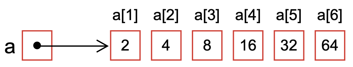
Fig. 4 Schematic of a 1-based array six-element array with name a.#
The items in an array are accessed using an index, an integer representing the item’s position in the collection. In most programming languages, arrays are zero-indexed, i.e., the first element in the array has an index of 0, the second element has an index of 1, and so on. However, arrays in Julia are one-based, i.e., the first element has an index 1, the second element has an index 2, etc.
Arrays can store large amounts of data because they allow fast access to any element using the index. Elements of an array are typically indexed using bracket notation in most languages such as Julia or Python:
# Define an array -
a = [2,4,8,16,32,64]

# What is the 3rd element of the array a?
i = 3
println("The third element of a = $(a[i])")
The third element of a = 8
However, array access uses parenthesis in niche systems, such as Matlab/Octave. Accessing individual elements or contiguous ranges of elements of an array is fast, but inserting or deleting elements from the middle of an array can be slow, as it requires shifting the elements to make room for the new element or closing the gap left by the deleted element.
Types of arrays: Vectors, Matrices, and d-dimensional arrays#
There are different sizes (types) of arrays, such as one-dimensional arrays (vectors), which store a linear sequence of elements, and multi-dimensional arrays, e.g., two-dimensional arrays (matrices) or arrays of arrays that store data in more complex structures.
In Julia, the size of an array and the type of data that will be stored in the array are declared when you initialize the array. For example, a 1-dimensional array of indefinite length that holds integers is declared as:
# Define an array arr
arr = Array{Int64,1}() # the array is empty

# When an array has an undefined length, we use the push! operation to add values
push!(arr,1); # adds a 1 to index 1
push!(arr,2); # adds a 2 to index 2
push!(arr,4); # adds a 4 to index 3

# print elements of the array -
println("Elements of arr = $(arr)")
Elements of arr = [1, 2, 4]
Of course, if you know how many elements you need the array to store beforehand, you can declare that when the array is constructed:
# Define an array arr
arr = Array{Int64,1}(undef, 10) # the array has 10 elements, each initialized to undefined

# When an array has a defined length, we use the = operation to add values
for i in 1:10
  arr[i] = 2^i # fills the array with powers of 2
end

# print elements of the array -
println("Elements of arr = $(arr)")
Elements of arr = [2, 4, 8, 16, 32, 64, 128, 256, 512, 1024]
Two-dimensional arrays follow a similar pattern when we declare the array; however, there is no direct equivalent to the push! operation for two- (or higher) dimensional arrays. Thus, when dealing with multi-dimensional arrays, we typically need to know the size of each dimension when we declare the array:
# Define a 2-dimensional array A
A = Array{Int64, 2}(undef, 4, 4) # array of Int's has 4 rows, 4 cols, initialized to undefined

# When an array has a defined length, we use the = operation to add values
# This creates an upper-triangular matrix with powers 2
for i in 1:4
  for j in 1:4
    if (i<=j)
      A[i,j] = 2^j # fills the array with powers of 2 along the col index
    else
      A[i,j] = 0 # adds a zero
    end
  end
end

# print elements of the array
A
4×4 Matrix{Int64}:
 2  4  8  16
 0  4  8  16
 0  0  8  16
 0  0  0  16
Stacks#
A stack data structure follows the last-in, first-out (LIFO) principle, the last element added to a stack will be the first element removed (Fig. 5). Unlike an array, you cannot access the elements of a stack by their index. Instead, elements are added to the top of the stack (also known as pushing) and removed from the top of the stack (also known as popping).
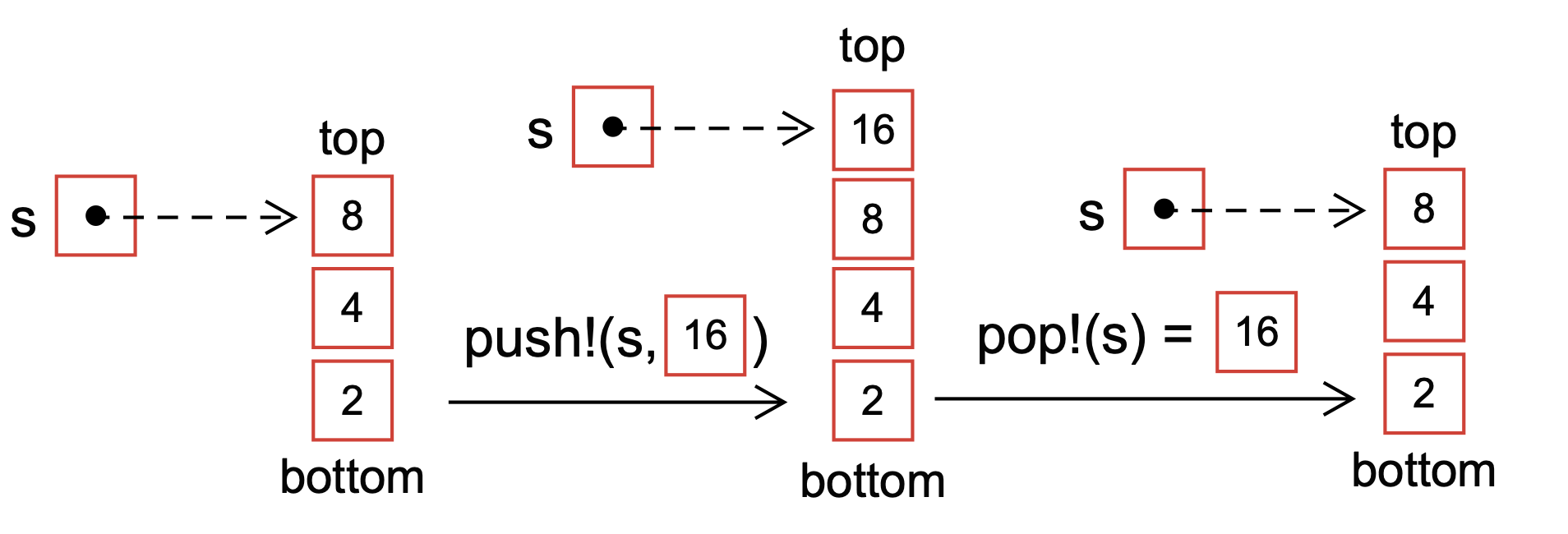
Fig. 5 Schematic of the push! and pop! operations for a stack s. Stacks follow the last-in, first-out paradigm. Thus, new elements are continually added to the top of the stack, while elements are drawn from the top (depicted with the dashed arrow).#
Stacks in Julia are implemented in the DataStructures.jl package:
using DataStructures # import the DataStructures package

# create an empty Stack that holds Int64 values
s = Stack{Int64}()

# add some values to the Stack using the push! operation
push!(s, 1);
push!(s, 2);
push!(s, 3);

# Grab a value from the Stack using the pop! operation
x = pop!(s);

# print x
println("What value did we get from the Stack = $(x)")
In this example, the elements 1, 2, and 3 are added to the stack s using the push! operation. The pop! operation removes the top element of the stack, i.e., the value 3 (the last item added); thus, pop! removes elements from the stack in the opposite order they were added.
Common uses of Stacks:#
Function call stack: In programming languages, the function call stack is typically implemented as a stack data structure. Each time a function is called, its information (such as local variables, parameters, and return address) is pushed onto the stack. When the function returns, its information is popped off the stack, allowing the program to resume execution from where it left off.
Undo/redo functionality: Many applications that allow users to undo and redo actions use a stack data structure to keep track of the actions. Each time a user acts, such as typing a letter or moving an object, the action is added to the stack. The most recent activity is popped off the stack and undone when the user chooses to undo an action. Similarly, the redo functionality pushes undone actions back onto the stack.
Expression evaluation: Stack data structures can also be used to evaluate mathematical expressions, such as those in postfix notation. Operands are pushed onto the stack in this case, and operators are applied to the most recently pushed operands. The result is then pushed back onto the stack until the entire expression has been evaluated.
Queues#
The queue data structure follows the first-in, first-out (FIFO) principle, the first element added to the queue will be the first element to be removed (Fig. 6). In a queue, elements are added to the bottom (also known as enqueuing) and removed from the top (also known as dequeuing).
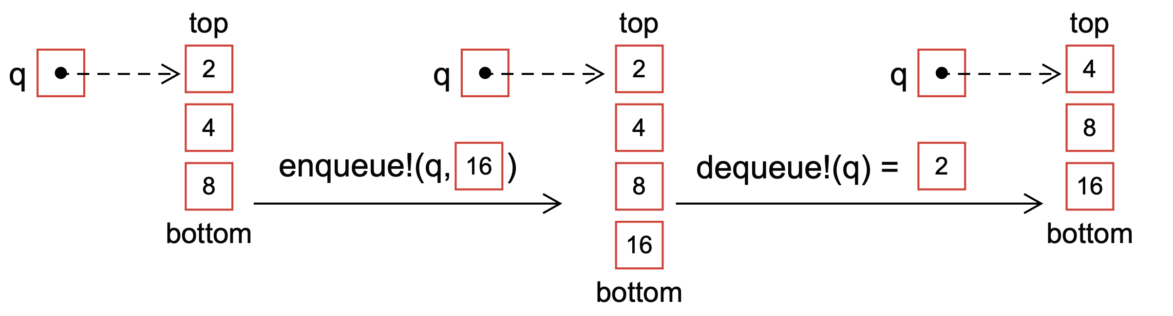
Fig. 6 Schematic of the enqueue! and dequeue! operations for a queue q. Queues follow the first-in, first-out paradigm. Thus, new elements are continually added to the bottom of the queue, while elements are drawn from the top (depicted with the dashed arrow).#
Queues in Julia are implemented by the DataStructures.jl package:
using DataStructures # import the DataStructures package

# create an empty Queue that holds Int64 values
q = Queue{Int64}()

# add some values to the Queue using the enqueue! operation
enqueue!(q, 1);
enqueue!(q, 2);
enqueue!(q, 3);

# Grab a value from the Queue using the dequeue! operation
x = dequeue!(q);

# print x
println("What value did we get from the Queue = $(x)")
In this example, the elements 1, 2, and 3 are added to the queue q in that order using the enqueue! operation. The dequeue! operation removes the top element from the queue, i.e., the value 1 (the first item added); dequeue! removes elements from the queue in the order they were added.
Common uses of Queues#
Job scheduling: Queues are often used in operating systems to manage tasks, such as running programs or printing documents. Each task is placed in a queue, and the operating system schedules tasks in the order they were added to the queue, allowing tasks to be processed in the order they were received.
Breadth-first search: In graph theory, the breadth-first search algorithm explores a graph by visiting all the vertices at a given level before moving on to the next level. This can be implemented using a queue data structure, where the vertices at each level are added to the queue in order and processed in that exact order.
Message passing: Queues are often used to pass messages between different parts of a system, such as between a producer and a consumer in a messaging system. Messages are added to the back of the queue by the producer and consumed from the front of the queue by the consumer. This allows the producer and consumer to operate at different speeds without the risk of messages being lost or overwritten.
In addition to the abovementioned applications, Queues are an ideal data structure for recursive parsing applications. Let’s build a recursive string parser using a Queue (Example 13):
Example 13 (Recursive descent string parser)
Develop a recursive parser that returns the words in a sentence as a Dict{Int64, String}, where the keys are the index of the word in the sentence, and the values are the words.
Test input: “you’ve got mail works alot better than it deserves to . “
Solution: We’ll encode the string we need to parse in a queue data structure. We’ll process each character until the queue is empty (base case): i) if the character is not the delimiter, then we’ll store it; ii) if the character is the delimiter, we’ll assemble all the characters that we stored into a string add to the external array.
Assumptions: This code assumes that the DataStructures.jl package has been installed; the DataStructures.jl implements the Queue data structure.
# load external packages -
using DataStructure

"""
    _recursive_parser(q::Queue, s::Array{Char,1}, a::Array{String,1}; delim = ' ')
"""
function _recursive_parser(q::Queue, s::Array{Char,1}, a::Array{String,1};
    delim = ' ')

    # base case: we have no more characters in the character_arr - we are done
    if (isempty(q) == true)
        return nothing
    else

        # grab the next_char -
        next_char = dequeue!(q)
        if (next_char == delim)

            # if we get here, then we have hit a delim character, this means we should
            # turn the characters in the s array into a word
            # join chars in the character array -
            word = join(s)
            if (isempty(word) == false)
                push!(a,word) # add that word to our word list -
            end

            # empty out the array of characters, because we may need it again
            empty!(s);
        else

            # if we get here, next_char is *not* the delim, so push next_char into the array
            # Why? we are collecting next_char until we hit a delim or hit the base case
            # When we hit a delim the characters in s can be joined to make a word
            push!(s, next_char)
        end

        # process the next character in the queue -
        _recursive_parser(q,s,a; delim = delim);
    end
end

"""
    recursive_parser(string::String; delim::Char=' ') -> Dict{Int64,String}
"""
function recursive_parser(string::String;
    delim::Char=' ')::Dict{Int64,String}

    # initialize -
    d = Dict{Int,String}()
    a = Array{String,1}()
    s = Array{Char,1}()
    q = Queue{Char}()
    counter = 0

    # build the Queue q that we are going to parse -
    character_arr = collect(string)
    for c ∈ character_arr
        enqueue!(q, c);
    end

    # recursive descent -
    _recursive_parser(q, s, a; delim = delim);

    # convert to dictionary for the output
    for item ∈ a
        d[counter] = item;
        counter += 1
    end

    # return -
    return d
end

# setup:
test_input = "you've got mail works alot better than it deserves to . "

# call -
d = recursive_string_parser(test_string);
Linked lists#
Linked lists are a common alternative to arrays because they can be resized easily; ndoes can be inserted or removed without moving the other nodes. A linked list is a linear data structure where each element, called a node, is a separate object that stores a data value and a reference (link) to the next node in the list (Fig. 7).
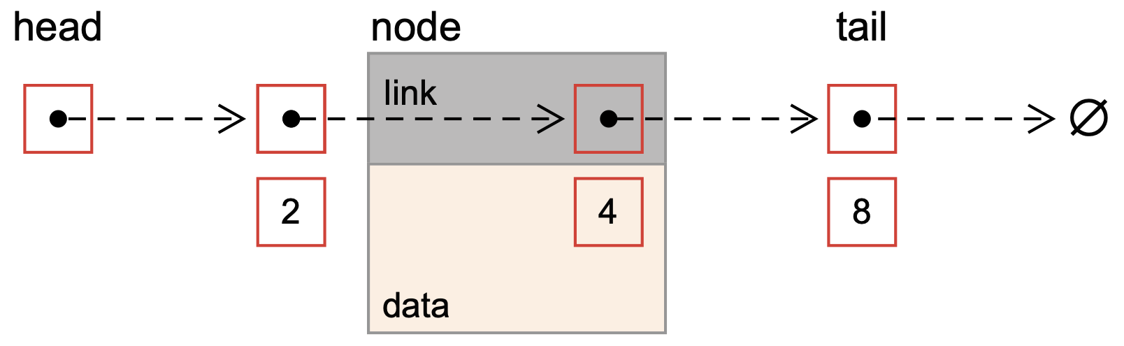
Fig. 7 Schematic of a singly linked list. Each node in the list has data, in this case, a queue data structure and a reference (link) to the next node in the list.#
There are two main types of linked lists: singly linked lists and doubly linked lists. In a singly linked list, each node has a reference to the next node in the list but not the previous one. On the other hand, each node connects to the next and previous nodes in a doubly linked list.
Common uses of linked lists#
Linked lists are often used when the data structure size is not known in advance or when the data needs to be inserted or removed frequently, as the time complexity for these operations is constant for a linked list.
Dynamic data structures: Linked lists are helpful when working with data structures that can change in size during runtime. Unlike arrays, linked lists can grow or shrink as needed without complex memory management or copying operations. This makes them helpful in implementing stacks, queues, and other dynamic data structures.
Memory allocation: In computer memory management, linked lists are used to keep track of free and allocated memory blocks. Each memory block is represented as a node in the list, with a pointer to the next block. This allows the system to find a suitable block for a new allocation quickly and to free up blocks when they are no longer needed efficiently.
Modeling hierarchical data: Linked lists can represent hierarchical data structures, such as trees and graphs. Each node in the list represents a tree node or graph vertex and contains a pointer to its children or neighbors. This allows the data to be stored and manipulated efficiently while maintaining the hierarchical structure.
Linked lists can also implement Stacks and Queues. Let’s consider an example Julia implementation of a stack-based upon a linked list (Example 14):
Example 14 (Linked-list implementation of a Stack)
Develop a stack data structure that holds characters using a linked list.
Solution: Let’s implement our character stack by defining the Node and Stack types and the push! and pop! operations in a file called Stack.jl (in the src directory):
"""
Mutable node type for the linked list stack implementation
"""
mutable struct Node

    # data
    value::Char
    next::Union{Nothing, Node}

    # constructor -
    Node() = new();
end

"""
Mutable stack type
"""
mutable struct Stack
    head::Union{Nothing, Node}
end

"""
    push!(stack::Stack, value::Char)

Implements the push! operation for our linked list stack
"""
function push!(stack::Stack, value::Char)

    # create a new node -
    new_node = Node()
    new_node.value = value;       # set the data value on the node
    new_node.next = stack.head;   # set the reference to the next item in the ll

    # set the head ot the stack to the new node
    stack.head = new_node
end

"""
    pop!(stack::Stack)

Implements the pop! operation for our linked list stack
"""
function pop!(stack::Stack)

    # if we don't have any more chars, then throw an error
    if stack.head === nothing # whay the === and not ==?
        throw("Stack is empty") # "throw" an error
    end

    # grabs the value held by the current head
    value = stack.head.value

    # updates the head reference to the next item in the stack
    stack.head = stack.head.next

    # return the char value
    return value
end
To build our stack, we can add the following code to a runme.jl file (in the root directory) where we have assumed our standard example/project structure (paths, packages, and our codes included in an Include.jl file in the root):
# include the Include -
include("Include.jl")

# create a new an empty stack -
s = Stack(nothing);

# add characters to the stack -
text = "Roomba!"
char_array = collect(text);
for c ∈ char_array
    push!(s,c)
end
source: Source code can be found in the CHEME-1800/4800 tree examples repository
Non-linear data structures#
Non-linear data structures store and manage data in more complex ways, allowing for faster access and manipulation of data, especially data with hierarchical relationships. However, non-linear data structures are typically more complex to construct and require more memory to store data. We’ll consider a few handy non-linear data structures, Dictionary and sets, Trees, and Graphs.
Dictionary and sets#
A dictionary stores key-value pairs, where each key value is unique. Dictionaries use a hash function to map keys (which can be a variety of types) to an array index. Thus, dictionaries have efficient lookup and insertion operations. Sets are similar to dictionaries but only store keys and do not have values associated with them.
Dictionaries are implemented in both Julia and Python as a Dict type; we’ve already seen several examples of Julia dictionaries when working with JSON, TOML and YAML files or other examples. Python dictionaries behave in a similar way as thier Julia counterparts, with one important exception: in Python > 3.7 dictionaries are ordered, while Julia dictionaries are always unordered.
Dictionaries are included in the standard libraries of Julia and Python; thus, they are available without importing external modules. Let’s look at an examples of dictionaries in Julia and Python:
# Initialize and empty dictionary, keys are strings, values can be anything
car = Dict{String,Any}()

# load key=value pairs into the dictionary
car["brand"] = "Ford"
car["model"] = "Mustang"
car["year"] = 1964
# Initialize and empty dictionary
car = {}

# Add data to car dictionary
car["brand"] = "Ford"
car["model"] = "Mustang"
car["year"] = 1964
Like dictionaries, both Julia and Python implement a Set type in their respective standard libraries. The Set type holds a unique collection of keys but does not associate these keys with any data:
# Initialize an empty set that stores strings
fruit = Set{String}()

# add items to a set using push!
push!(fruit, "Apple")
push!(fruit, "Pear")
push!(fruit, "Mango")
# Initialize an empty set
fruit = set()

# Add data to the fruit set
fruit.add("Apple")
fruit.add("Pear")
fruit.add("Mango")
In both Julia and Python, the Set type is unordered; thus, unlike Arrays, Stacks or Queues, the order in which items are added to the set is not maintained.
Hash functions#
The exciting thing about a dictionary implementation, e.g., the Dict type in Julia, is the fast lookup enabled by mapping an arbitrary key to an array index. This mapping is enabled using a hash function.
A hash function takes an input value, e.g., a string key, and returns a fixed-size string or number (hash value). The same key information will always produce the same index output, but even a small change to the input will have a very different result. In the case of a dictionary, when a key is passed to the hash function, it calculates a hash value, which is then used as the index at which the corresponding data value is stored in an array.
Let’s look at some pseudo code for a simple hash function (Algorithm 1):
Algorithm 1 (Simple Hash Function)
Inputs String key, a size parameter, a \(\beta\) factor
Outputs hash
Initialize
set hash \(\leftarrow{0}\)
set \(L\leftarrow\text{length}(\text{key})\)
Main
for \(i\in{1,\dots,L}\)
hash \(\leftarrow\left(\text{hash}\times\beta+\text{key}[i]\right)\) % size
Return hash
Algorithm 1 is a variant of Horner’s hashing method when \(\beta\) = 31. The modulo operator % computes the remainder, e.g., the expression 7 % 3 evaluates to 1. The modulo % operation with size ensures that the output hash value is a valid index within the array.
Example 15 (Hashing example)
Compute the hash value for the key = CHEME-1800 for an array of size of 1000 and expansion factor \(\beta\) = 31.
Solution: We implemented Algorithm 1 in Julia. The myhash function takes a string key as input and has optional default values for the \(\beta\) and size parameters.
"""
    myhash(key::String, β::Int64, size::Int64)::Int64

Convert a String `key` to `Int` for an array of type `size`:
"""
function myhash(key::String; β::Int64 = 31, size::Int64 = 1000)::Int64

    # initialize -
    hash = 0
    L = length(key)

    # main loop -
    for i ∈ 1:L
        hash = (hash*β + convert(Int, key[i])) % size
    end

    # return -
    return hash
end
To call this myhash function with the key = CHEME-4800, we issue the commands in the REPL:
julia> key = "CHEME-4800"
julia> hashvalue = myhash(key);
The myhash implementation above should return a value of 153 for the key = CHEME-4800.
Trees#
Trees are widely used non-linear data structures that encode hierarchical structures in data that are composed of nodes and edges (Fig. 8).
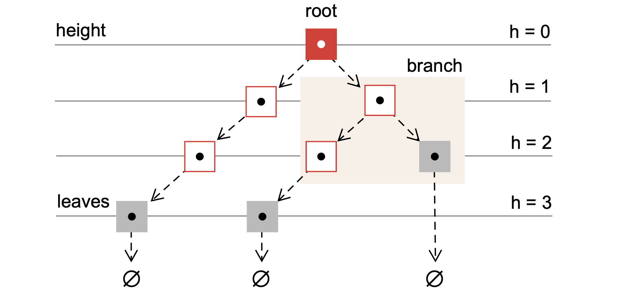
Fig. 8 Schematic of a tree data structure. Each node in the tree holds some data and references (links) to its children. If a node does not have children, it is a leaf node. The topmost node in the tree is the root node.#
Each node may have one or more child nodes, and each child node has one or more sub-children, and so on. The topmost node, which has no parent, is called the root node, while nodes with no children are called leaf nodes. The edges connecting the nodes represent the relationships between the nodes. Finally, the number of levels of a tree is called the height of the tree. Let’s define some properties of a complete k-ary tree (Definition 3):
Definition 3 (Children and nodes of a full k-ary tree)
Let \(\mathcal{T}\) be a full k-ary tree with height \(h\) where each node of \(\mathcal{T}\) has \(k\) children. The tree’s height \(\mathcal{T}\) will be defined as the maximum number of edges from the root node to a tree leaf. Further, let the root node of \(\mathcal{T}\) have an index \(0\).
Then, the indices of the children of node \(i\), denoted by the set \(\mathcal{C}_{i}\), are given by:
and the total number of nodes of tree \(\mathcal{T}\) with branched height \(h\), denoted by \(N_{h}\), is given by:
where \(N_{h}\) includes the final layer of leaves.
Common uses for trees#
Trees are ubiquitous in computing; trees are used in a huge variety of applications:
Organizing and searching data: Trees commonly store and organize hierarchical data, such as file systems, organizational charts, and website navigation menus. The hierarchical structure of a tree makes it easy to search for specific items and perform operations like adding, deleting, or updating elements.
Implementing algorithms: Many algorithms in computer science are implemented using tree data structures. For example, binary search trees enable efficient searching for an item in a sorted list. In contrast, heaps and priority queues efficiently extract the maximum or minimum element from a collection.
Modeling real-world phenomena: Trees can be used to model many real-world phenomena, such as family trees, taxonomies, and decision trees. Decision trees are commonly used in machine learning to model decision-making processes and classify data based on binary decisions.
One interesting application of trees beyond what was listed above is to diagram function calls in a recursive function. Let’s reimagine the recursive computation of the Fibonacci series that uses memoization (Example 16):
Example 16 (Recursive Fibonacci and Memoization)
One tool to diagram how a recursive function works is by developing a call tree. Previously, we constructed a recursive implementation of the Fibonacci function, which computed the Fibonacci sequence. The call tree for recursive fibonacci(4) is shown in (Fig. 9):
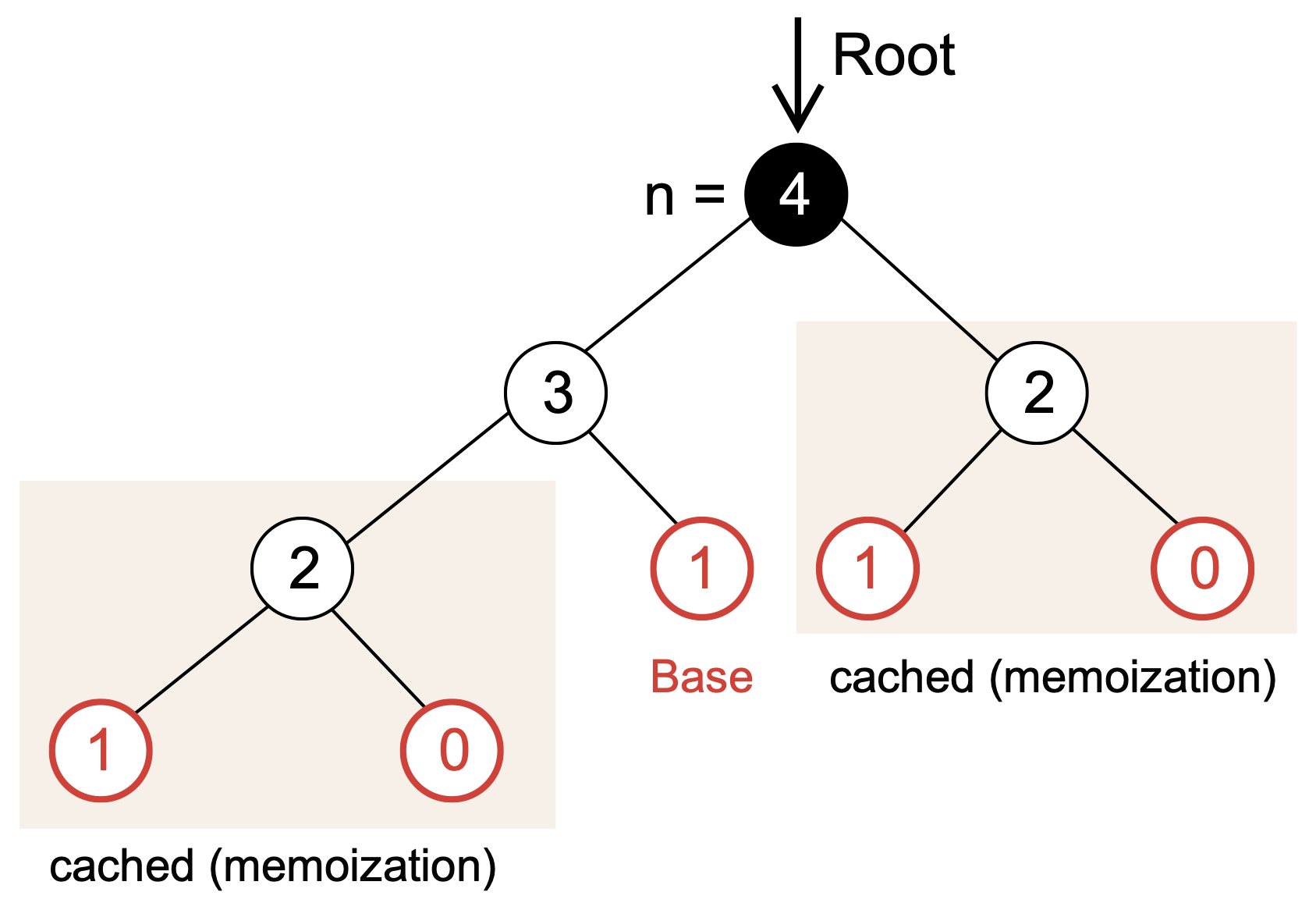
Fig. 9 Schematic of the function call tree for the recursive implementation of the fibonacci function with \(n=4\).#
Representation of Trees#
Trees can be implemented in a variety of ways. Suppose we’re interested in a k-ary tree \(\mathcal{T}\) where each node has \(k\)-children. Two of the most common representations are Array-based and Adjacency list representations.
In an array-based representation of a tree, each node is assigned an index in an array that stores the tree data. Consider a 3-ary (ternary) tree describing possible prices for a commodity as a function of time (Example 17):
Example 17 (Ternary commodity price tree array-representation)
Construct a ternary pricing tree that describes a two-time step projection of a commodity price using an array-based tree representation.
Let the current price of a commodity, e.g., a raw material required for a chemical process, be given by \(P_{o}\). Assume that at each subsequent time-step in the future, the price can increase by \(r_{+}\) = 2%, stay the same \(r_{0}\) = 0%, or decrease by \(r_{-}\) = 1%.
Solution: The height of the tree \(h\) will be the number of future time-steps. Thus, from Definition 3, we know the total number of nodes in the tree (length of the storage array) is \(N_{2} = 13\). Further, we know the relationship between the parent price \(P_i\) and children prices is given by:
We can now develop a build method that takes information about the tree and returns a list of the values of the commodity price at each node in the tree.
Preconditions: The ArrayBasedTernaryCommodityPriceTree mutable type has been defined outside of the build function.
"""
    build(type::Type{ArrayBasedTernaryCommodityPriceTree};
        h::Int64 = 1, price::Float64 = 1.0, u::Float64 = 0.02, d::Float64 = 0.01) -> ArrayBasedTernaryCommodityPriceTree
"""
function build(type::Type{ArrayBasedTernaryCommodityPriceTree};
    h::Int64 = 1, price::Float64 = 1.0, u::Float64 = 0.02, d::Float64 = 0.01)::ArrayBasedTernaryCommodityPriceTree

    # initialize -
    model = ArrayBasedTernaryCommodityPriceTree(); # build an empty tree model -
    Nₕ = sum([3^i for i ∈ 0:h]) # compute how many nodes we have in the tree
    P = Dict{Int64,Float64}()

    # setup Δ - the amount the price moves up, or down -
    Δ = [u,0,-d];

    # set the root price -
    P[0] = price

    # fill up the array -
    for i ∈ 0:(Nₕ - 3^h - 1)

        # what is the *parent* price -
        Pᵢ = P[i]

        # Compute the children for this node -
        Cᵢ = [j for j ∈ (3*i+1):(3*i+3)];
        for c ∈ 1:3 # for each node (no matter what i) we have three children

            # what is the child index?
            child_index = Cᵢ[c]

            # compute the new *child* prive
            P[child_index] = Pᵢ*(1+Δ[c])
        end
    end

    # set the price data on the model -
    model.data = P;

    # return -
    return model
end
To call this build function, we issue the commands in the REPL:
julia> include("Include.jl") # assumes standard CHEME-1800/4800 code format
julia> Pₒ = 75.00; # set the initial price
julia> m = build(ArrayBasedTernaryCommodityPriceTree; h = 2, price = Pₒ); # build the tree
source: Source code can be found in the CHEME-1800/4800 tree examples repository
In an adjacency list representation, the list of children at index \(i\), denoted by \(\mathcal{C}_{i}\), is still given by Eqn. (6). However, instead of storing the edges and data in the same array, the edge connectivity is stored in an array or dictionary, and the data is stored in a separate data structure.
Let’s reimagine the ternary commodity price model in the Adjacency list format (Example 18):
Example 18 (Ternary commodity price tree adjacency list)
Construct a ternary pricing tree that describes a two-time step projection of a commodity price using an adjacency list representation.
Let the current price of a commodity, e.g., a raw material required for a chemical process, be given by \(P_{o}\). Assume that at each subsequent time-step in the future, the price can increase by 2%, stay the same, or decrease by 1%.
Solution: The height of the tree \(h\) will be the number of future time-steps. Thus, from Definition 3 we know the total number of nodes in the tree (length of the storage array) is \(N_{2} = 13\). Further, we know the relationship between the parent price \(P_i\) and children’s prices will be the same as the array-based representation.
We can now develop a build method that takes information about the tree and returns a list of the values of the commodity price at each node in the tree, along with a data structure holding information about the tree connectivity.
Preconditions:
The
AdjacencyBasedTernaryCommodityPriceTreemutable tree type has been defined outside of thisbuildfunction.
"""
    build(type::Type{AdjacencyBasedTernaryCommodityPriceTree};
        h::Int64 = 1, price::Float64 = 1.0, u::Float64 = 0.02, d::Float64 = 0.01) -> AdjacencyBasedTernaryCommodityPriceTree
"""
function build(type::Type{AdjacencyBasedTernaryCommodityPriceTree};
    h::Int64 = 1, price::Float64 = 1.0, u::Float64 = 0.02, d::Float64 = 0.01)::AdjacencyBasedTernaryCommodityPriceTree

    # initialize -
    model = AdjacencyBasedTernaryCommodityPriceTree(); # build an emprt tree model
    Nₕ = sum([3^i for i ∈ 0:h]) # compute how many nodes we have in the tree
    P = Dict{Int64,Float64}() # use Dict for zero-based array hack. Hold price information
    connectivity = Dict{Int64, Array{Int64,1}}() # holds tree connectivity information

    # setup Δ - the amount the price moves up, or down -
    Δ = [u,0,-d];

    # set the root price -
    P[0] = price

    # build connectivity -
    for i ∈ 0:(Nₕ - 3^h - 1)

        # what is the *parent* price
        Pᵢ = P[i]

        # Compute the children for this node -
        Cᵢ = [j for j ∈ (3*i+1):(3*i+3)];
        connectivity[i] = Cᵢ # stores the children indices of node i

        # cmpute the prices at the child nodes
        for c ∈ 1:3 # for each node (no matter what i) we have three children

            # what is the child index?
            child_index = Cᵢ[c]

            # compute the new price for the child node
            P[child_index] = Pᵢ*(1+Δ[c])
        end
    end

    # set the data, and connectivity for the model -
    model.data = P;
    model.connectivity = connectivity;

    # return -
    return model;
end
To call this build function, we issue the commands in the REPL:
julia> include("Include.jl") # assumes standard CHEME-1800/4800 code format
julia> Pₒ = 75.00; # set the initial price
julia> m = build(AdjacencyBasedTernaryCommodityPriceTree; h = 2, price = Pₒ); # build the tree.
source: Source code can be found in the CHEME-1800/4800 tree examples repository
Graphs#
A graph is a data structure consisting of a finite set of vertices (also called nodes) and a set of edges connecting these vertices. Edges can be directed (also called arcs) or undirected and can carry data (Fig. 10).
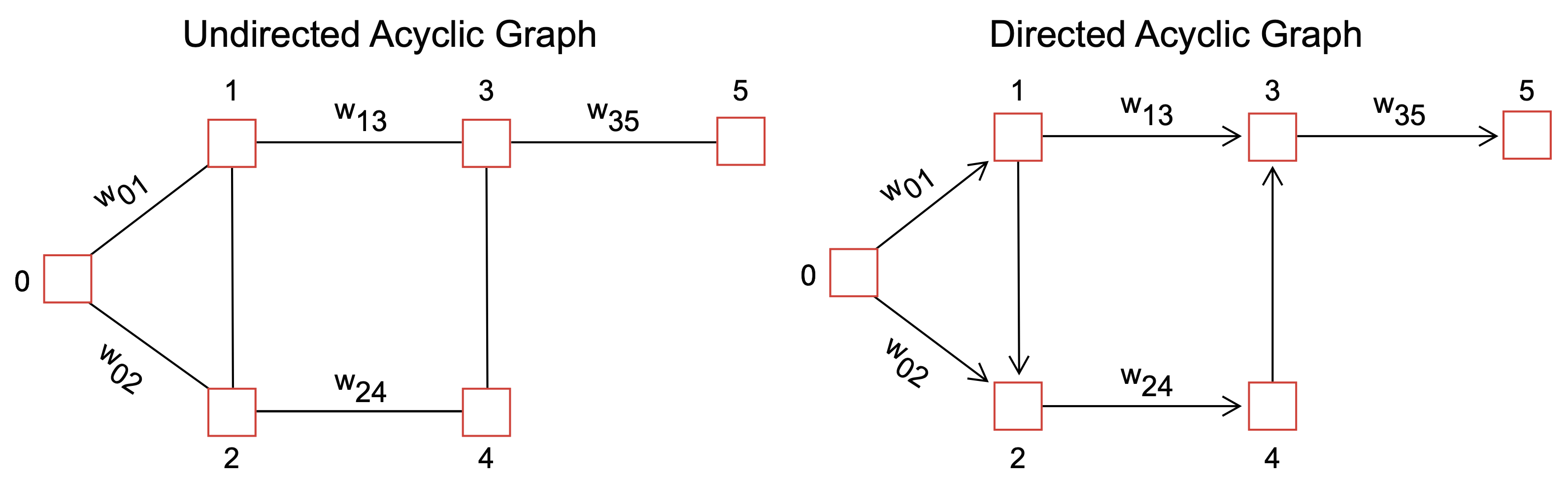
Fig. 10 Schematic of a graph data structures. Nodes in a graph hold references (called links or edges) to other nodes in the graph. The edges between node \(j\) and \(j\), which can be undirected (left) or directed (right), can carry data (called edge weights, \(w_{ij}\)) representing many different quantities, e.g., degree of interaction, physical distances, travel times, financial values, etc.#
Graphs represent real-world situations like networks, maps, and social relationships. They are commonly used to describe relationships between data and to solve problems such as finding the shortest path between two nodes. Formally, graphs are defined in Definition 4:
Definition 4 (Definition and properties of Graphs)
A simple graph \(\mathcal{G}\) is composed of a set of vertices \(\mathcal{V}\) and edges \(\mathcal{E}\) such that there is at most one edge between vertices \(v_{i}\in\mathcal{V}\) and \(v_{j}\in\mathcal{V}\), and there are no edges that connect a vertex to itself (self-loop).
The edges in a graph can be directed and undirected:
In a directed graph, the edges have a direction and connect one vertex to another. The edges are often used to represent relationships or dependencies between the vertices. For example, in a social network, the vertices might represent people, and the directed edges might represent friendships, with the edge pointing from the person to their friend.
In an undirected graph, the edges have no direction and connect pairs of vertices. These edges represent connections or relationships between symmetrical vertices, such as friendships.
A graph \(\mathcal{G}\) is said to be connected if there is at least one path between vertices \(v_{i}\in\mathcal{V}\) and \(v_{j}\in\mathcal{V}\), where a path is defined as a sequence of vertices in which each successive vertex (after the first) is connected to its predecessor.
Connection between trees and graphs#
Graphs are used to model hierarchical relationships, but we have already seen that Trees can also be used to model hierarchical relationships. What is the difference between Trees and Graphs?
Structure: A tree is a type of graph with a specific structure. Trees are connected acyclic graphs, where only one path exists between any two nodes. In contrast, a graph can have cycles and may not be connected. Root node: A tree has a root node, the topmost node in the tree. Every other node in the tree is connected to it in some way. In a graph, there is no concept of a root node.
Direction: A tree is a directed graph, which means that every edge has a direction pointing from parent to child nodes. In a graph, edges may be directed or undirected and can point to any node.
Complexity: Trees are simpler than graphs because of their restricted structure. They have a unique path between any two nodes, which makes them easy to traverse and search. Conversely, graphs can be more complex and challenging to analyze because of their potentially cyclic and non-linear structure.
Representation of Graphs#
Similar to the Representation of Trees, graphs can be represented using Array and Adjacency list formats. The adjacency array for a graph is a two-dimensional array, i.e., a matrix instead of a vector (Definition 5):
Definition 5 (Adjacency matrix for graph \(\mathcal{G}\))
An adjacency matrix \(\mathcal{A}\) representation of a graph \(\mathcal{G} = (\mathcal{V},\mathcal{E})\) is a \(\dim\mathcal{V}\times\dim\mathcal{V}\) matrix holding integer or floating point values. The entry for row \(i\) and column \(j\) of the matrix \(\mathcal{A}\), denoted \(a_{ij}\in\mathcal{A}\), describes the connection between vertices \(v_{i}\in\mathcal{V}\) and \(v_{j}\in\mathcal{V}\).
Unweighted: If there is an edge connecting \(v_{i}\in\mathcal{V}\) and \(v_{j}\in\mathcal{V}\) and graph \(\mathcal{G}\) is unweighted, then \(a_{ij}=\)
1(true) , otherwise \(a_{ij}=\)0(false).Weighted: In cases where the edges of graph \(\mathcal{G}\) have weights, if there is an edge connecting \(v_{i}\in\mathcal{V}\) and \(v_{j}\in\mathcal{V}\) and graph \(\mathcal{G}\) is weighted, then \(a_{ij}=w_{ij}\), otherwise \(a_{ij}=\)
0(false), where \(w_{ij}\in\mathbb{R}\) denotes the weight of the edge connecting \(v_{i}\in\mathcal{V}\) and \(v_{j}\in\mathcal{V}\).
On the other hand, the adjacency list format for a graph \(\mathcal{G}\) is structured in a similar way as a tree (Definition 6):
Definition 6 (Adjacency list for graph \(\mathcal{G}\))
An adjacency list for a graph \(\mathcal{G} = (\mathcal{V},\mathcal{E})\) is a \(\dim\mathcal{V}\) dictionary \(d\), where the ith entry points to the children indices of vertex \(v_{i}\in\mathcal{V}\), denoted by set \(\mathcal{C}_{i}\). In other words, \(d_{i}\rightarrow\mathcal{C}_{i}\). There is a single entry in dictionary \(d\) for each vertex in graph \(\mathcal{G}\).
Depth-first graph traversal#
Depth-first traversal is a graph traversal algorithm that starts at a source vertex and visits vertices by exploring as far as possible along each branch before backtracking. Depth-first is often implemented using recursion but can also be implemented iteratively. A recursive depth-first traversal approach is outlined in Algorithm 2:
Algorithm 2 (Reversive depth-first traversal)
Inputs A graph \(\mathcal{G} = (\mathcal{V},\mathcal{E})\)
Initialize
set \(\text{visited}\leftarrow\text{Set{Vertex}}()\)
Depth-first traversal
DFS(\(\mathcal{G},v,\text{visited}\))
if \(v\in\text{visited}~\text{is}~\text{false}\)
\(\text{visited}\leftarrow\text{add}(\text{visited},v)\)
set \(\mathcal{C}\leftarrow\text{children}(\mathcal{G},v)\)
for \(c\in\mathcal{C}\)
DFS(\(\mathcal{G},c,\text{visited}\))
Main
for \(v\in\mathcal{V}\)
DFS(\(\mathcal{G},v,\text{visited}\))
How does depth-first traversal work?#
In Algorithm 2, \(\mathcal{G}\) is the graph (or tree) to be traversed, and start is the starting node for the traversal. Algorithm 2 uses a set visited to keep track of the nodes that have already been visited (to avoid visiting the same node twice).
Algorithm 2 calls the DFS procedure with the graph G, the start node, and the visited set as arguments. The DFS procedure then adds the current node to the visited set, processes it, and recursively calls itself for each unvisited child c of the current node. The recursion continues until all nodes have been visited.
Some of the most common uses of depth-first traversal are:
Pathfinding: Depth-first traversal can be used to find a path between two nodes in a graph. It is beneficial when the graph is a maze or a grid, as it can explore all possible paths from a starting point until it reaches the goal.
Cycle detection: Depth-first traversal can detect cycles in a graph. The graph contains a cycle if a back edge is encountered during the traversal.
Tree traversal: Depth-first traversal traverse a tree. In a tree, there is only one path from the root to any node, so the traversal can be done recursively by visiting the left subtree, the right subtree, and the root.
Breadth-first graph traversal#
Breadth-first traversal is a graph traversal algorithm that visits vertices in order of their distance from a source vertex. Breadth-first starts at a source vertex and explores all the vertices at the same level before moving on to the next level. A breadth-first traversal approach is outlined in Algorithm 3.
Algorithm 3 (Breadth-first traversal)
Inputs A graph \(\mathcal{G} = (\mathcal{V},\mathcal{E})\)
Initialize
set \(\text{visited}\leftarrow\text{Set{Vertex}}()\)
set \(\text{queue}\leftarrow\text{Queue{Vertex}}()\)
Breadth-first traversal
BFS(\(\mathcal{G}\), \(v\))
\(\text{queue}\leftarrow\text{enqueue}(\text{queue},v)\)
\(\text{visited}\leftarrow\text{add}(\text{visited},v)\)
while \(\text{queue}\) is not empty
set \(\text{current}\leftarrow\text{dequeue}(\text{queue})\)
set \(\mathcal{C}\leftarrow\text{children}(\text{current})\)
for \(c\in\mathcal{C}\)
if \(c\in\text{visited}~\text{is}~\text{false}\)
\(\text{queue}\leftarrow\text{enqueue}(\text{queue},c)\)
\(\text{visited}\leftarrow\text{add}(\text{visited},c)\)
Main
set \(\text{start}\leftarrow\text{start}(\mathcal{G})\)
BFS(\(\mathcal{G}\), \(\text{start}\))
How does breadth-first traversal work?#
In Algorithm 3, \(\mathcal{G}\) is the graph (or tree) to be traversed, and start is the starting node for the traversal. The algorithm uses a queue queue to keep track of the nodes to be visited next. The set visited is used to keep track of the nodes that have already been visited (which avoids visiting the same node twice).
Algorithm 3 starts by adding the start node to the visited set and enqueuing it onto the queue. Then, while queue is not empty, it dequeues the next node, which we call current, processes it and adds its unvisited children to the visited set and enqueues them onto queue. Algorithm 3 continues until the queue is empty and all nodes have been visited.
Some of the most common uses of breadth-first traversal are:
Shortest path: Breadth-first traversal can be used to find the shortest path between two nodes in an unweighted graph. Since it explores all the vertices at a given distance before moving to the next distance, it guarantees that the first time a node is visited, it is via the shortest path.
Web crawling: Breadth-first traversal can be used to crawl the web or any other network of interconnected data. By starting at a particular node and visiting all its neighbors before moving on to the neighbors of its neighbors, the traversal can be used to search for data systematically.
Social networking analysis: Breadth-first traversal can be used to analyze social networks, such as Facebook or Twitter, by starting at a particular user and visiting all their friends before moving on to the friends of their friends.
Decision making: Breadth-first traversal can be used to perform decision-making tasks, such as chess or game AI. By exploring all the possible moves that can be made in a game, the traversal can be used to identify the best move to make next.
Summary#
In this set of lectures, we introduced the concept of data structures and their application in various computing tasks.
Linear data structures are data structures that store data in a linear sequence, such as arrays, stacks, and queues. They are used to store and access data in a sequential manner.
Non-linear data structures are data structures that store data in a non-linear manner, such as trees and graphs. They are used to represent hierarchical relationships and complex networks of data.
Data structures are ways of organizing and storing data in a computer so that it can be accessed and modified efficiently. Different data structures are suited to various applications; some are highly specialized for specific tasks. In this lecture, we introduced several common data structures that will be important as we transition to applications.